← Eyal Merhavi · Labelings, models, and gauge theory
Chapter 1 of Labelings, models, and gauge theory, rendered from the executed notebook. Code cells and their outputs are shown as they ran.
Run this chapter in your browser ↗ · Source on GitHub ↗
Runs on JupyterLite. The first time, it downloads Python and its libraries (about 40 MB).
Chapter 1 — Labelings, reframings and classes
In Chapter 0 every edge of a currency market carried an exchange rate. When a country redenominated its currency, many rates changed at once, but no arbitrage opportunity appeared or disappeared. The rates were a description; the arbitrage was the content.
This chapter takes that idea and strips it down to its skeleton, so that it works for any group of labels, not just exchange rates. The labels might be coin flips (), clock hands (angles), shuffles of three cards (permutations), or the relative orientations of cameras (3D rotations). In every case the same three ingredients appear:
- labels on the edges of a graph,
- products of labels around loops,
- a freedom to change conventions at each vertex, which changes the labels but not the loop products (up to a twist we'll meet for non-commuting groups).
Nothing in this chapter is random. Probability arrives in Chapter 2.
What you'll learn
- the precise definitions of board, labeling, walk product, reframing and class;
- which functions of a labeling survive every reframing, and why traces appear for non-commuting groups;
- how to count classes, and how to pick one canonical representative of each (tree normal form).
Prerequisites: Chapter 0 (helpful, not required); basic group theory (groups, conjugation, conjugacy classes).
import itertools
import numpy as np
import matplotlib.pyplot as plt
import plotly.graph_objects as go
from IPython.display import HTML

from lgt import *
from lgt import viz

viz.use_style()
rng = np.random.default_rng(1)
1. Boards
We need a place to put labels. A graph alone is almost enough, but we will also want to single out some short loops as "elementary" (the little squares of a grid, for instance). So we bundle a graph with a chosen list of closed walks.
Definition (board, glossary 1.1–1.3). A board consists of
- a finite connected graph with vertex set and edge set ;
- a list of closed walks in that graph, called faces.
Every edge can be walked in two directions, and . We write for the set of all directions (), and for a direction we write for the same edge walked the other way.
Which closed walks count as faces is a choice we make when we build the board, much like choosing which pixels count as "neighbours" in an image model. On a grid the natural choice is the unit squares.
In code (and in the pictures) each edge is stored with one
reference direction
,
drawn as a small arrow. This is pure bookkeeping: the other direction is
always available too. A walk is stored as a list of steps
(e, sign), where sign = +1 walks edge
e along its arrow and sign = -1 walks it
against the arrow.
tri = Board.triangle()
grid = Board.grid(4, 3)
torus = Board.grid(3, 3, periodic=True)
for X in (tri, grid, torus):
    print(X)
Board('triangle': 3 vertices, 3 edges, 1 faces)
Board('4x3 grid': 12 vertices, 17 edges, 6 faces)
Board('3x3 periodic grid': 9 vertices, 18 edges, 9 faces)
Three boards we'll use throughout. The right-hand picture is a window cut through the middle of the wrap-around edges. Look at its borders: an edge that leaves through the right side comes back in through the left side, and one that leaves through the top comes back in at the bottom. The partial squares along the borders are pieces of the same wrapped faces. Gluing left to right and top to bottom turns the grid into the surface of a doughnut, so we call it a torus.
fig, axs = plt.subplots(1, 3, figsize=(13, 4.3))
viz.draw_board(axs[0], tri, vertex_labels=["0", "1", "2"], title="triangle: 3 edges, 1 face")
viz.draw_board(axs[1], grid, title="4×3 grid: 17 edges, 6 faces")
viz.draw_board(axs[2], torus, title="3×3 periodic grid (torus): 18 edges, 9 faces")
plt.show()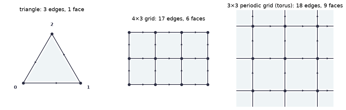
A face is a list of steps. Notice the two -1 signs in
the grid's first face: going counter-clockwise around a unit square, the
top and left edges are walked against their arrows.
print("triangle face (steps):  ", tri.faces[0], "  vertices:", tri.walk_vertices(tri.faces[0]))
print("first grid face (steps):", grid.faces[0], "  vertices:", grid.walk_vertices(grid.faces[0]))
triangle face (steps): [(0, 1), (1, 1), (2, 1)] vertices: [0, 1, 2, 0]
first grid face (steps): [(0, 1), (3, 1), (7, -1), (1, -1)] vertices: [0, 1, 5, 4, 0]
Recap. A board is a connected graph plus a list of designated closed walks (faces). Each edge has two directions; code stores one reference direction per edge and records walks as
(edge, ±1)steps.
Check yourself
- How many vertices, edges and faces does an grid (no wrap-around) have?
Answer
vertices; edges ( horizontal edges in each of rows, same for columns); faces.
- And an torus (with )?
Answer
vertices; edges (every vertex has one edge going right and one going up); faces.
- Why do we store a face as a list of steps rather than as a set of vertices?
Answer
A face is a closed walk: it has an order, a direction, and a starting point, and all three will matter once labels are multiplied around it. Also, on a small torus two different edges can join the same pair of vertices, so a list of vertices would not even say which edges are used.
2. Labelings and their products
2.1 Label groups
Definition (label group, glossary 2.1). A label group is any group. Its elements are the labels we will put on edges. Our running examples:
| group | elements | multiplication | how we draw a label |
|---|---|---|---|
| ("coins") | ordinary product | edges are thick and gold | |
| addition mod 3 | clock hand at | ||
| ("clocks") | angles | addition mod | clock hand at angle |
| ("shuffles") | permutations of | composition | cycle notation, e.g. |
| ("cameras") | rotations of 3D space | composition | rotation angle |
The first three are abelian (the order of multiplication doesn't matter); the last two are not. For permutations we compose like functions: means "apply first, then ".
S = S3()
fmt = lambda x: viz.format_label(S, x)          # S3 element -> cycle notation
x, y = 2, 1                                      # x = (12), y = (23)
print(f"x = {fmt(x)},  y = {fmt(y)}")
print(f"xy = {fmt(S.mul(x, y))},  yx = {fmt(S.mul(y, x))}   <- different: S3 is not abelian")
x = (12), y = (23)
xy = (123), yx = (132) <- different: S3 is not abelian
2.2 Labelings
Definition (labeling, glossary 2.2). A labeling is a function with
Read as a converter from the conventions at to the conventions at . Walking the edge backwards must undo the conversion, which is what the rule says. (In Chapter 0: if a dollar buys 3.7 shekels, a shekel buys dollars.)
Because the reverse label is forced, a labeling is the same thing as one label per edge, so the set of all labelings is . In code, a labeling is an array with one entry per edge (for its reference direction).
2.3 Walk products, loop products, face products
Definition (walk product, glossary 2.3). For a walk that takes the directions in order, its walk product is
Definition (loop product, face product, defect; glossary 2.4–2.5). If is closed and starts and ends at , is a loop product at . The loop product of a face is its face product . A face with (not the identity) is a defect.
Here is a random labeling of the 4×3 grid. Each clock hand is a label. Each face is coloured by its face product: pale means identity (angle ), and as the angle goes around the circle the colour runs through blues and purples to dark, then through reds and tans back to pale. The teal loop goes around a block of faces.
G = U1()
U = random_labeling(G, grid, rng)      # U: one angle per edge, an array of shape (|E|,)
block = grid.walk([0, 1, 2, 6, 10, 9, 8, 4, 0])   # vertex list -> list of steps

fig, ax = plt.subplots(figsize=(6.5, 4.8))
viz.draw_board(ax, grid, U, G, highlight_walk=block, title="a U(1) labeling and a loop")
plt.show()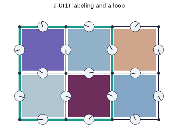
For an abelian group, the product around the block equals the product of the four face products inside it: every interior edge is walked once in each direction and cancels. Let's check.
inside = [i for i, (c, mu, nu) in enumerate(grid.meta["face_anchor"]) if c[0] < 2 and c[1] < 2]
fp = face_products(G, grid, U)                       # one angle per face
print("loop product around the block:   ", round(float(walk_product(G, grid, U, block)), 4))
print("product of the 4 faces inside it:", round(float(G.prod(fp[inside])), 4))
loop product around the block: 0.9569
product of the 4 faces inside it: 0.9569
For a non-abelian group, order matters, and two more facts are worth seeing at work.
Fact 1.1 (reversal). Walking a walk backwards inverts its product: if is walked backwards, then .
Why: .
Moving the starting point of a loop changes its product by a conjugation: if the loop is (first a walk from to , then a walk back to ), then starting at gives .
US = random_labeling(S, grid, rng)                 # an S3 labeling of the same grid
while S.chi(walk_product(S, grid, US, block)) != 0:  # redraw until the product is a 3-cycle
    US = random_labeling(S, grid, rng)              # (a swap is its own inverse: less instructive)
fwd = walk_product(S, grid, US, block)
bwd = walk_product(S, grid, US, grid.reverse_walk(block))
shifted = walk_product(S, grid, US, block[1:] + block[:1])      # same loop, starting at vertex 1
print(f"around the block from 0:    {fmt(fwd)}")
print(f"backwards:                  {fmt(bwd)}   (inverse of {fmt(fwd)} is {fmt(S.inv(fwd))})")
print(f"same loop, starting at 1:   {fmt(shifted)}   (a conjugate of {fmt(fwd)})")
around the block from 0: (132)
backwards: (123) (inverse of (132) is (123))
same loop, starting at 1: (123) (a conjugate of (132))
2.4 Consistent labelings
Definition (consistent, glossary 2.6). A labeling is consistent if every loop product is the identity. In Chapter 0 this was "no arbitrage".
Checking every loop sounds expensive, but on a plain grid it's enough to check the faces:
Fact 1.2 (faces suffice on a grid). On a grid without wrap-around, a labeling is consistent if and only if it has no defects.
Why, roughly: every loop on a flat grid can be shrunk across faces one at a time, and each step changes the loop product only by a face product (and conjugations). Section 7 shows that this fails on a torus.
Let's check it by brute force: all coin labelings of the 3×3 grid.
Z = Z2()
small = Board.grid(3, 3)
Us = all_labelings(Z, small)                          # shape (4096, 12)
no_defects = ~defects(Z, small, Us).any(axis=1)
consistent = is_consistent(Z, small, Us)
print(f"{len(Us)} labelings, {no_defects.sum()} with no defects, "
      f"{consistent.sum()} consistent; the two lists agree: {(no_defects == consistent).all()}")
4096 labelings, 256 with no defects, 256 consistent; the two lists agree: True
An application: cameras. Suppose each vertex is a camera with an unknown orientation , and for each pair of cameras we measure their relative rotation . Exact measurements give a consistent labeling: around any loop the 's cancel. Real measurements are noisy, so the loop products become small non-identity rotations. Recovering the from noisy 's is called synchronization, and it is used in 3D reconstruction from photos and in cryo-electron microscopy.
R = SO3()
cams = Board.complete(4)                                   # 4 cameras, all pairs compared
O = R.uniform(rng, cams.n_vertices)                        # true orientations, unknown in practice
s, t = cams.edges[:, 0], cams.edges[:, 1]
U_exact = R.mul(O[s], R.inv(O[t]))                         # U(s->t) = O_s O_t^{-1}
noise = np.array([R.about_axis(rng.normal(size=3), rng.normal(0, 0.03)) for _ in s])
U_noisy = R.mul(U_exact, noise)
for name, X in [("exact", U_exact), ("noisy", U_noisy)]:
    ang = np.degrees(R.rotation_angle(face_products(R, cams, X)))
    print(f"{name:5}  rotation angle of each triangle's face product (degrees):", np.round(ang, 2))
exact rotation angle of each triangle's face product (degrees): [0. 0. 0. 0.]
noisy rotation angle of each triangle's face product (degrees): [1.6 2.74 1.12 3.48]
Recap. A labeling puts a group element on every edge direction, with reverse = inverse. Multiplying labels along a walk gives its walk product; around a closed walk it's a loop product, around a face a face product. Reversing a walk inverts the product; moving a loop's start conjugates it. A labeling is consistent when every loop product is the identity; on a plain grid, that's the same as having no defects.
Check yourself
- For , what is a face product in words?
Answer
It is where is the number of edges around the face. So a face is a defect exactly when an odd number of its edges carry .
- For an abelian group, does the starting point of a loop affect its product?
Answer
No. Moving the start conjugates the product, and in an abelian group .
- In the camera example, why is the exact labeling consistent?
Answer
Around a closed walk the product is : every inner pair cancels.
3. Reframings
The camera example already contains the key idea. The labels were built from one choice per vertex. If you rotated all your notes about camera (you decided "up" means something else for that camera), every label touching would change, yet nothing physical about the cameras would.
Definition (reframing, glossary 3.1–3.2). A reframing is a function . It acts on a labeling by
The set of all reframings, , is a group under vertex-by-vertex multiplication; we call it the reframing group.
Each label is a converter between the conventions at its two endpoints, so a change of convention at either endpoint enters it: on the left, on the right. (Check that the reverse direction stays the inverse: is indeed the inverse of .)
The payoff of this exact shape is that along a walk the inner factors telescope:
Here and are the labels of two consecutive steps.
Fact 1.3 (how reframing moves products; glossary 3.5). If is a walk from to , a reframing changes its product to . In particular a loop product at becomes : it is conjugated.
For an abelian group, conjugation does nothing, so loop products are untouched. For a non-abelian group the loop product can change, but only within its conjugacy class. Here is an labeling of the triangle, before and after a reframing:
U = np.array([2, 1, 1])                 # labels (12), (23), (23) on 0->1, 1->2, 2->0
h = np.array([1, 3, 0])                 # reframing: h(0)=(23), h(1)=(123), h(2)=e
U2 = reframe(S, tri, U, h)
for name, X in [("before", U), ("after ", U2)]:
    w = face_products(S, tri, X)[0]
    print(f"{name}: labels {[fmt(x) for x in X]}   loop product {fmt(w):5}   "
          f"fixed points of loop product: {S.chi(w):.0f}")
print(f"check: h(0) w h(0)^-1 = {fmt(S.conj(h[0], face_products(S, tri, U)[0]))}")
before: labels ['(12)', '(23)', '(23)'] loop product (12) fixed points of loop product: 1
after : labels ['(123)', '(12)', 'e'] loop product (13) fixed points of loop product: 1
check: h(0) w h(0)^-1 = (13)
Every label changed and the loop product changed from to . But both are swaps of two cards: same conjugacy class, same number of fixed points.
Frozen faces, spinning edges
For an abelian group the effect is striking. Below, a labeling of a 3×3 grid is hit by a smoothly varying reframing: every vertex slowly turns its own "zero direction". Watch the clock hands spin while the face colours do not move at all. The faces are what the labeling means; the hands are how it is written down.
G = U1()
U = random_labeling(G, small, np.random.default_rng(7))
anim = viz.animate_reframing(small, G, U, n_frames=36, figsize=(4.2, 4.2), interval=110)
HTML(anim.to_jshtml())
Reframings compose the way you'd hope: doing and then is the same as doing the single reframing (multiply vertex by vertex). This is what it means for the reframing group to act on labelings.
h1, h2 = random_reframing(S, grid, rng), random_reframing(S, grid, rng)
one_by_one = reframe(S, grid, reframe(S, grid, US, h1), h2)
combined = reframe(S, grid, US, S.mul(h2, h1))
print("h1 then h2  ==  h2·h1 :", np.array_equal(one_by_one, combined))
h1 then h2 == h2·h1 : True
Recap. A reframing changes conventions vertex by vertex and acts by . Along a walk the inner factors cancel, so only the endpoints feel it; a loop product at gets conjugated by . For abelian groups, loop products don't change at all.
Check yourself
- Let be constant, for every . What does it do to a labeling when is abelian? When it isn't?
Answer
Abelian: , so nothing at all. Non-abelian: it conjugates every label by the same .
- Write out the telescoping for a three-step walk .
Answer
.
- In the camera example, the exact labeling was . Express it as a reframing of something.
Answer
It is the reframing applied to the identity labeling (every label ): .
4. Invariants and loop observables
Since reframings only change the description, the interesting functions of a labeling are the ones that ignore them.
Definition (invariant, glossary 3.4). An invariant is a function such that whenever is a reframing of .
For abelian , Fact 1.3 hands us invariants for free: every loop product. For non-abelian a loop product only survives up to conjugation, so we need a way to read off a number that doesn't notice conjugation.
Definition (class function, glossary 3.6). A class function is a function with for all .
The most useful class function is the trace of a
matrix, since
.
Each of our groups comes with one, available as G.chi:
| itself | |
| , | |
| number of fixed points (the trace of the permutation matrix) | |
| trace |
Definition (loop observable, glossary 3.7). For a closed walk and a class function , the loop observable is .
Fact 1.4. Every loop observable is an invariant.
Why: the loop product gets conjugated (Fact 1.3) and doesn't notice conjugation. Let's test it with random rotations on the 3×3 grid: the face products change, their traces don't. A walk that is not closed gives no invariant.
U = random_labeling(R, small, rng)
h = random_reframing(R, small, rng)
U2 = reframe(R, small, U, h)
fp, fp2 = face_products(R, small, U), face_products(R, small, U2)
boundary = small.walk([0, 1, 2, 5, 8, 7, 6, 3, 0])
open_walk = small.walk([0, 1, 2])
print("face products unchanged?        ", np.allclose(fp, fp2))
print("traces of face products unchanged?", np.allclose(R.chi(fp), R.chi(fp2)))
print("trace around the boundary:  before %.4f  after %.4f" % (
    R.chi(loop_product(R, small, U, boundary)), R.chi(loop_product(R, small, U2, boundary))))
print("trace along an open walk:   before %.4f  after %.4f" % (
    R.chi(walk_product(R, small, U, open_walk)), R.chi(walk_product(R, small, U2, open_walk))))
face products unchanged? False
traces of face products unchanged? True
trace around the boundary: before -0.8745 after -0.8745
trace along an open walk: before -0.2796 after -0.8780
Recap. An invariant is a function of a labeling that every reframing leaves alone. Loop products are invariants for abelian groups; for non-abelian groups we apply a class function such as the trace, giving loop observables .
Check yourself
- Is "the label on edge " an invariant?
Answer
No. Reframing at either endpoint of changes it (unless is trivial).
- Is "the number of defects" an invariant?
Answer
Yes. Each face product is conjugated, and if and only if , so a face is a defect before the reframing exactly when it is one after.
- Is the rotation angle of an loop product an invariant?
Answer
Yes: it is a function of the trace (), hence a class function of the loop product.
5. Classes, and how many there are
Definition (class, glossary 3.3). The class of a labeling is
Two labelings are in the same class exactly when they describe the same thing in different conventions. Invariants are precisely the functions of the class.
How many classes are there? For a finite group, there are labelings and reframings. If the only reframing that fixed a labeling were the trivial one ( for all ), each class would have members. But for an abelian group the constant reframings ( for all ) do nothing, and on a connected board they are the only reframings that fix a labeling. That gives:
Fact 1.5 (counting classes, abelian). For a finite abelian on a connected board, every class has exactly members, so there are classes. The exponent is the number of independent cycles of the graph.
We check this by brute force: list every labeling, sort them into classes, count.
def count_classes(G, X):
    Us = all_labelings(G, X)
    return len(Us), class_ids(G, X, Us).max() + 1

for G in (Z2(), ZN(3)):
    for X in (Board.triangle(), Board.grid(2, 2), Board.grid(3, 2), Board.grid(2, 2, periodic=True)):
        n, k = count_classes(G, X)
        print(f"{G.name:3} {X.name:18}  labelings {n:5}   classes {k:4}   "
              f"|G|^(E-V+1) = {G.order ** X.cycle_rank}")
Z2 triangle labelings 8 classes 2 |G|^(E-V+1) = 2
Z2 2x2 grid labelings 16 classes 2 |G|^(E-V+1) = 2
Z2 3x2 grid labelings 128 classes 4 |G|^(E-V+1) = 4
Z2 2x2 periodic grid labelings 256 classes 32 |G|^(E-V+1) = 32
Z3 triangle labelings 27 classes 3 |G|^(E-V+1) = 3
Z3 2x2 grid labelings 81 classes 3 |G|^(E-V+1) = 3
Z3 3x2 grid labelings 2187 classes 9 |G|^(E-V+1) = 9
Z3 2x2 periodic grid labelings 6561 classes 243 |G|^(E-V+1) = 243
For a non-abelian group, some labelings are fixed by more reframings than others (for instance the identity labeling is fixed by every constant reframing), so classes have different sizes and the simple division fails. A standard counting argument (Burnside's lemma) gives the answer:
Fact 1.6 (counting classes, any finite ). With , the number of classes is , where is the set of elements commuting with .
For abelian every is all of and this collapses to .
def burnside(G, b):
    els = G.elements()
    commuting = [sum(bool(G.equal(G.mul(g, x), G.mul(x, g))) for x in els) for g in els]
    return sum(c ** b for c in commuting) // len(els)

for X in (Board.triangle(), Board.grid(2, 2), Board.grid(3, 2)):
    n, k = count_classes(S, X)
    print(f"S3 {X.name:10}  labelings {n:6}   classes {k:3}   Burnside formula {burnside(S, X.cycle_rank)}")
S3 triangle labelings 216 classes 3 Burnside formula 3
S3 2x2 grid labelings 1296 classes 3 Burnside formula 3
S3 3x2 grid labelings 279936 classes 11 Burnside formula 11
On the triangle, has 3 classes: one per conjugacy class of the loop product (identity, swaps, 3-cycles). Here are the class sizes on the 3×2 grid, which are indeed unequal:
ids = class_ids(S, Board.grid(3, 2), all_labelings(S, Board.grid(3, 2)))
sizes, how_many = np.unique(np.bincount(ids), return_counts=True)
for sz, m in zip(sizes, how_many):
    print(f"{m:3} classes of size {sz}")
1 classes of size 7776
4 classes of size 15552
3 classes of size 23328
3 classes of size 46656
Seeing classes: the triangle with clock labels
For there are infinitely many labelings, but on the triangle we can see all of them. A labeling is three angles , one per edge, so the set of labelings is a cube whose opposite sides are glued together (an angle of is an angle of ). Every invariant is a function of the loop product , so each class is a level set of that sum: a flat sheet that gets cut into pieces where it hits the cube's walls.
The figure shows three classes, coloured by their loop product, together with 600 random reframings of one labeling (black dots). Look at where the dots land: all on one colour, spread over all of its pieces. One labeling's reframings fill out its entire sheet, and never leave it. Collapsing each sheet to a single point leaves one number, the loop product: the space of classes is a circle.
def plane_in_cube(s):
    """Corners of the polygon where the plane x+y+z = s cuts the cube [0, 2π]^3."""
    corners = [np.array(c, float) for c in itertools.product([0, TAU], repeat=3)]
    pts = []
    for a, b in itertools.combinations(corners, 2):
        sa, sb = a.sum(), b.sum()
        if np.sum(a != b) == 1 and sa != sb and (sa - s) * (sb - s) <= 0:
            pts.append(a + (s - sa) / (sb - sa) * (b - a))
    pts = np.unique(np.round(pts, 9), axis=0)
    u, v = np.array([1, -1, 0]) / 2**0.5, np.array([1, 1, -2]) / 6**0.5   # axes in the plane
    d = pts - pts.mean(axis=0)
    return pts[np.argsort(np.arctan2(d @ v, d @ u))]

def sheet_traces(c, color, name):
    """All pieces of the class 'loop product = c' as Plotly meshes."""
    out = []
    for k in range(3):                                   # the sum can be c, c+2π or c+4π
        P = plane_in_cube(c + k * TAU)
        if len(P) < 3:
            continue
        n = len(P)
        out.append(go.Mesh3d(x=P[:, 0], y=P[:, 1], z=P[:, 2], i=[0] * (n - 2),
                             j=list(range(1, n - 1)), k=list(range(2, n)), color=color,
                             opacity=0.45, name=name, showlegend=(k == 0), flatshading=True))
    return out
cmap = plt.get_cmap("twilight")
classes = [0.6, 2.4, 4.4] # three loop products (radians)
traces = []
for c in classes:
r, g, b, _ = cmap(c / TAU)
traces += sheet_traces(c, f"rgb({255*r:.0f},{255*g:.0f},{255*b:.0f})",
f"class with loop product {c / np.pi:.2f}π")
theta = np.array([1.0, 2.0, 2.4 - 3.0 + TAU]) # a labeling with loop product 2.4
hs = rng.uniform(0, TAU, size=(600, 3)) # 600 random reframings
orbit = reframe(U1(), tri, theta, hs) # shape (600, 3)
traces.append(go.Scatter3d(x=orbit[:, 0], y=orbit[:, 1], z=orbit[:, 2], mode="markers",
marker=dict(size=2, color="#2b2d42"), name="reframings of one labeling"))edges = [(a, b) for a, b in itertools.combinations(itertools.product([0, TAU], repeat=3), 2)
if sum(x != y for x, y in zip(a, b)) == 1]
for a, b in edges: # wireframe of the cube
traces.append(go.Scatter3d(x=[a[0], b[0]], y=[a[1], b[1]], z=[a[2], b[2]], mode="lines",
line=dict(color="#8d99ae", width=2), showlegend=False, hoverinfo="skip"))
ax = dict(range=[0, TAU], tickvals=[0, np.pi, TAU], ticktext=["0", "π", "2π"])
fig = go.Figure(traces)
fig.update_layout(height=620, margin=dict(l=0, r=0, t=30, b=0), legend=dict(x=0, y=1),
scene=dict(xaxis=dict(title="θ(0→1)", **ax), yaxis=dict(title="θ(1→2)", **ax),
zaxis=dict(title="θ(2→0)", **ax), aspectmode="cube"))
fig.show()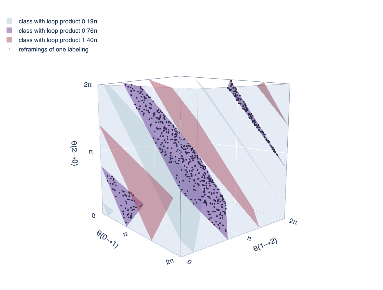
Recap. The class of is everything reframings can turn it into; invariants are functions of the class. For a finite abelian group there are classes, all the same size. For non-abelian groups the sizes differ and Burnside's formula counts them. For on the triangle, classes are sheets in a glued cube, labelled by one angle.
Check yourself
- How many classes does have on the 3×3 grid (no wrap-around)? What determines a class?
Answer
, so classes. There are exactly 4 faces, and by Facts 1.2 and 1.5 a class is pinned down by which of the 4 faces are defects ( possibilities, all of which occur).
- For on the triangle, name a representative labeling of each of the 3 classes.
Answer
Put labels on the three edges with , , or . Their loop products are , which lie in the three different conjugacy classes.
- In the cube picture, how many dimensions does a class have, and why?
Answer
Two. A reframing has 3 angles, but adding the same angle at all three vertices does nothing (abelian group), leaving directions of motion. That is the same count, , as in Fact 1.5.
6. Tree normal form: one representative per class
A class is a large set. It would be convenient to pick one canonical member, the way you'd reduce a fraction to lowest terms. Chapter 0 did this for currencies by quoting every rate in dollars along a tree of exchanges.
Construction. Fix a spanning tree and a root vertex . For each vertex , let be the walk product from to along the tree. Reframing by makes every tree edge carry the identity: for a tree edge we have , so the new label is .
Fact 1.7 (tree normal form; glossary 3.8). Every class contains a labeling that is the identity on every edge of . On each of the other edges, its label is the loop product of that edge's fundamental cycle: go from to in the tree, cross the edge , return from to in the tree. For abelian this representative is unique; for non-abelian it is unique up to conjugating all labels by one common element.
The free labels are exactly the numbers that Fact 1.5 counted.
G = U1()
U = random_labeling(G, grid, rng)
Un, h, tree = tree_normal_form(G, grid, U)        # Un = reframe(G, grid, U, h)
cycles = grid.fundamental_cycles()                # {non-tree edge: its fundamental cycle}
e0 = sorted(cycles, key=lambda e: len(cycles[e]))[len(cycles) // 2]
ok = all(G.equal(Un[e], loop_product(G, grid, U, cycles[e])) for e in cycles)
print(f"{len(tree)} tree edges, {len(cycles)} free edges; "
      f"free labels = fundamental loop products: {ok}")
11 tree edges, 6 free edges; free labels = fundamental loop products: True
Left: the random labeling. Right: its tree normal form. The grey tree edges all point their hands at angle (the identity). The face colours are identical in the two pictures, because it's the same class. The teal walk is the fundamental cycle of one free edge, and that edge's clock shows its loop product.
fig, axs = plt.subplots(1, 2, figsize=(12, 4.6))
viz.draw_board(axs[0], grid, U, G, title="a labeling U")
viz.draw_board(axs[1], grid, Un, G, tree_edges=tree, highlight_walk=cycles[e0],
               title="its tree normal form (tree in grey)")
plt.show()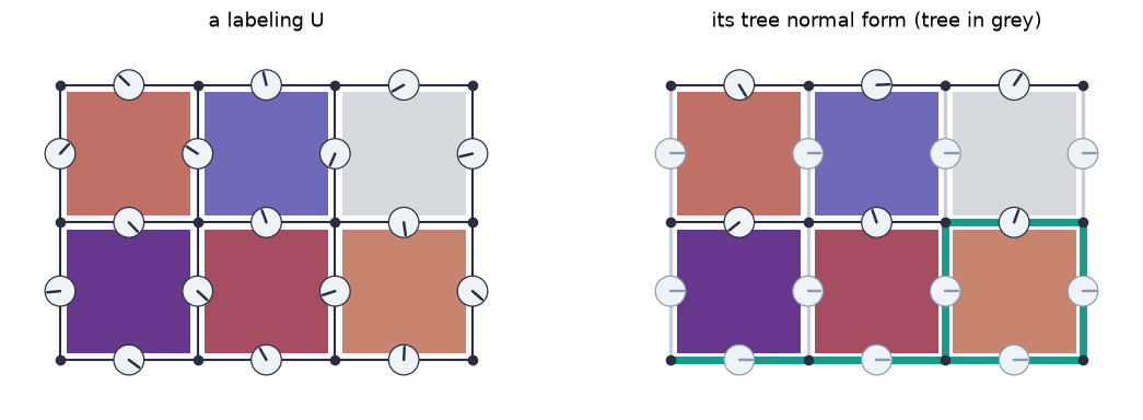
Recap. Choosing a spanning tree and pushing all labels off it gives a canonical representative of each class: identity on the tree, fundamental loop products on the remaining edges.
Check yourself
- Two labelings have the same tree normal form (same tree and root, abelian ). What can you conclude?
Answer
They are in the same class: each is a reframing of the common normal form, and reframings can be undone and composed.
- Why is the non-abelian normal form only unique up to a common conjugation?
Answer
The reframings that keep the tree at the identity are exactly the constant ones, . They conjugate every free label by the same .
7. The torus: when faces don't tell the whole story
Fact 1.2 said that on a plain grid, "no defects" means "consistent". On a torus it doesn't. Take the coin group on the 3×3 torus and flip the three horizontal edges that cross one vertical line (a "seam"). Each face either misses the seam or crosses it twice, so no face is a defect. But a loop that goes once around the torus horizontally crosses the seam exactly once.
T, Z = Board.grid(3, 3, periodic=True), Z2()
U = identity_labeling(Z, T)
seam = [T.meta["edge_index"][(v, 0)] for v in (0, 3, 6)]   # horizontal edges from column 0 to 1
U[seam] = -1
row = T.walk([0, 1, 2, 0])                                  # once around, horizontally
col = T.walk([0, 3, 6, 0])                                  # once around, vertically
print("defects:", int(defects(Z, T, U).sum()),
      "  | around a row:", int(loop_product(Z, T, U, row)),
      "  | around a column:", int(loop_product(Z, T, U, col)),
      "  | consistent?", bool(is_consistent(Z, T, U)))
defects: 0 | around a row: -1 | around a column: 1 | consistent? False
Left: the seam (gold edges are ); every face is pale, so there are no defects. Right: the same labeling with the bottom row's loop (once around the torus) in teal. It uses exactly one seam edge, so its loop product is .
fig, axs = plt.subplots(1, 2, figsize=(10, 5))
viz.draw_board(axs[0], T, U, Z, title="a seam: no defects")
viz.draw_board(axs[1], T, U, Z, highlight_walk=row, title="...but this loop has product −1")
plt.show()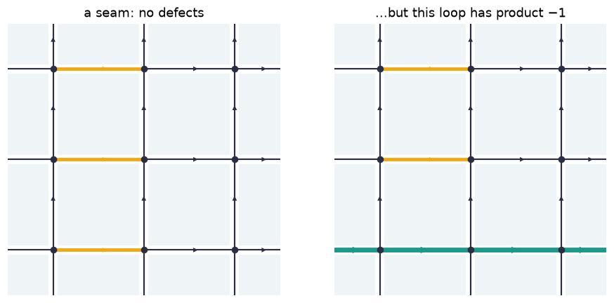
Counting confirms there's room for exactly this kind of thing. The 3×3 torus has independent cycles but only 9 faces, and the faces aren't even independent:
Fact 1.8 (faces on a torus). For abelian on a periodic grid, the product of all face products is the identity. So the faces carry only independent pieces of information, and the remaining are the loop products around the two directions of the torus. In particular there are classes with no defects at all.
Why the first part: every edge borders exactly two faces and is walked once in each direction, so in an abelian group every label cancels against its inverse.
T4 = Board.grid(4, 4, periodic=True)
U = random_labeling(U1(), T4, rng)
everything = U1().prod(face_products(U1(), T4, U))
print("4×4 torus, random U(1) labeling: product of all 16 face products is the identity?",
      bool(U1().is_identity(everything)))
Us = all_labelings(Z, T)                                   # all 2^18 coin labelings
ids = class_ids(Z, T, Us)
clean = ~defects(Z, T, Us).any(axis=1)
print(f"{len(Us)} labelings, {ids.max() + 1} classes, "
      f"{len(np.unique(ids[clean]))} classes with no defects (Fact 1.8 predicts 2^2 = 4)")
4×4 torus, random U(1) labeling: product of all 16 face products is the identity? True
262144 labelings, 1024 classes, 4 classes with no defects (Fact 1.8 predicts 2^2 = 4)
Recap. On a torus, a labeling can be defect-free and still have non-identity loop products around the holes. For abelian groups the faces carry independent pieces of information and the two winding loops carry the rest.
Check yourself
- On an torus with , how many classes have no defects?
Answer
: one for each choice of the two winding loop products.
- Where does the argument "product of all face products " use that is abelian?
Answer
To cancel a label against its inverse, the two must be brought next to each other in the product. That reordering is only allowed when is abelian; for non-abelian the faces' products start at different vertices and come in different orders.
- On the 3×3 torus, describe a coin labeling whose loop product is around both a row and a column but which has no defects.
Answer
Combine two seams: flip the three horizontal edges crossing one vertical line and the three vertical edges crossing one horizontal line. Each face still crosses each seam zero or two times.
Chapter recap
- A board is a connected graph with a chosen list of closed walks called faces.
- A labeling puts a group element on every direction, with reverse = inverse. Multiplying along a walk gives its walk product; around closed walks, loop products; around faces, face products.
- A reframing acts by . Walk products only feel it at their endpoints; loop products are conjugated.
- Invariants are the functions that every reframing leaves alone. Loop products for abelian , and loop observables for any class function , are invariants.
- The class is the set of all reframings of . For finite abelian there are classes.
- Tree normal form picks one representative per class: identity on a spanning tree, fundamental loop products elsewhere.
- On a torus, faces don't see everything: the loops around the holes carry two extra invariants.
Dictionary
| Our term | Other names you'll meet |
|---|---|
| board | lattice, 2-complex; "spacetime" in physics |
| face | plaquette (physics), 2-cell (topology) |
| label group | gauge group (physics), gain group (gain graphs), structure group (geometry) |
| labeling | gauge field, configuration, link variables (physics); gain function (gain graphs); connection (geometry, synchronization) |
| walk product | parallel transport, Wilson line (physics); gain of a walk |
| loop product | holonomy, monodromy |
| face product | plaquette variable (physics); curvature, field strength (geometry) |
| defect | vortex, frustrated plaquette (spin glasses) |
| consistent | flat, pure gauge (physics); balanced (gain graphs); cycle-consistent (vision) |
| reframing | gauge transformation (physics); switching (gain graphs) |
| reframing group | gauge group (in mathematics) |
| class | gauge orbit, physical configuration (physics); switching class (gain graphs) |
| invariant | gauge-invariant observable |
| loop observable | Wilson loop |
| tree normal form | gauge fixing, maximal-tree or axial gauge |
What's next
Interlude (optional, recommended). Why should edges carry labels at all? The interlude Why the labels are forced puts values on vertices and shows that comparing neighbors requires a label on the edge between them. For the circle group, that is electromagnetism.
So far a labeling was just given to us. In Chapter 2 we choose labelings at random, with a distribution that prefers few and mild defects. That raises an immediate question: if the labels are random, but only their class has meaning, does the redundancy we found here distort the probabilities? (It doesn't. The class counts of Section 5 and the tree normal form of Section 6 are both part of the reason.)