← Eyal Merhavi · Labelings, models, and gauge theory
Chapter 2 of Labelings, models, and gauge theory, rendered from the executed notebook. Code cells and their outputs are shown as they ran.
Run this chapter in your browser ↗ · Source on GitHub ↗
Runs on JupyterLite. The first time, it downloads Python and its libraries (about 40 MB).
Chapter 2 — Models: putting a probability distribution on labelings
Take the grid wrapped around in both directions, so that it becomes a torus as in chapter 1. It has 4 vertices, 8 edges and 4 faces. Flip a fair coin for every edge and write or on it. How many faces do you expect to be defects, meaning faces whose face product is ? Now suppose someone tells you that defects are expensive, and that a labeling with many of them should be less likely. How would you tilt the coins?
This chapter answers that question, and the answer is the central object of the whole course. We stop looking at one labeling and start looking at a probability distribution over all labelings. We call that distribution a model. Everything that comes later (averages, correlations, and in chapter 5 even "dynamics") will be read off from the model alone.
What you'll learn
- What it means to pick a group element "uniformly at random", and why that needs a compact group.
- How a cost on faces and a single number (the stiffness) turn the uniform distribution into a model.
- Why the redundancy from chapter 1 (reframings) does no harm, and why, on a planar grid with the coin group, the faces are independent coins.
Prerequisites: chapter 1 (boards, labelings, face products, reframings, classes, tree normal form). Chapter 0 helps for intuition but is not required.
import numpy as np
import matplotlib.pyplot as plt
from lgt import *
from lgt import viz

viz.use_style()
rng = np.random.default_rng(2)
1. Choosing a label "uniformly at random"
Before we can make labelings unequally likely, we need to know what equally likely means. For a fair coin this is obvious: and each get probability . For a general group the right notion is this: picking an element at random and then multiplying it by any fixed element should not change the odds.
Definition (uniform distribution, glossary 4.1). Let be a group. A uniform distribution on is a probability distribution on such that, for every fixed and every set ,
In words: if is drawn from , then is drawn from too.
Our examples:
- Coin group : each element gets probability .
- (integers mod ): each element gets probability .
- Circle (angles mod ): the angle is uniform on .
- Rotations : a "uniformly random rotation". As we'll see in a moment, this is not what you might first guess.
Fact 2.1 (when a uniform distribution exists). A uniform distribution on exists exactly when is compact, and then it is unique. For us, "compact" means one of two things: finite (like , , the permutations ), or a closed and bounded set of matrices (like the circle or the rotations ).
The exchange rates of chapter 0 live in , which is not compact. Picking a "uniformly random positive number" is as impossible as picking a uniformly random integer. That is why chapter 0 had no randomness in it.
for G in [Z2(), ZN(5), U1()]:
    print(f"{str(G):>4}: eight uniform draws ->", np.round(G.uniform(rng, 8), 2))
Z2: eight uniform draws -> [-1 1 1 1 1 -1 1 1]
Z5: eight uniform draws -> [1 3 4 3 4 0 4 0]
U1: eight uniform draws -> [1.73 4.13 3.53 0.94 2.72 4.21 2.66 3.98]
A surprise: a uniform rotation does not have a uniform angle
Every rotation of 3D space turns by some angle about some axis. You might expect a uniformly random rotation to have a uniformly random angle. It doesn't.
Fact 2.2 (angle of a uniform rotation). If is drawn from the uniform distribution on , its rotation angle has density .
Why, roughly: the rotations by a fixed angle form a whole sphere's worth of axes, and that sphere gets bigger as grows. Large angles have "more room", so tiny rotations are rare.
The figure checks two things. The filled histogram is uniform rotations; look at how it follows the dark curve and not the flat dashed line. The outlined histogram is the same rotations each multiplied by one fixed rotation . It is indistinguishable from the first, which is exactly the defining property of "uniform".
R = SO3()
w = R.rotation_angle(R.uniform(rng, 200_000))
g = R.about_axis([1, 2, 0], 2.0)                       # one fixed rotation
w_g = R.rotation_angle(R.mul(g, R.uniform(rng, 200_000)))
om = np.linspace(0, np.pi, 300)
fig, ax = plt.subplots(figsize=(7.5, 3.6))
ax.hist(w, bins=60, density=True, alpha=0.5, label="uniform rotations $R$")
ax.hist(w_g, bins=60, density=True, histtype="step", lw=2, label="the same, each turned into $gR$")
ax.plot(om, (1 - np.cos(om)) / np.pi, color=viz.INK, lw=2, label=r"$(1-\cos\omega)/\pi$")
ax.axhline(1 / np.pi, ls="--", color=viz.MUTED, label="flat: what you might have guessed")
ax.set(xlabel=r"rotation angle $\omega$", ylabel="density", xlim=(0, np.pi))
ax.legend(frameon=False, fontsize=9, loc="upper left")
plt.show()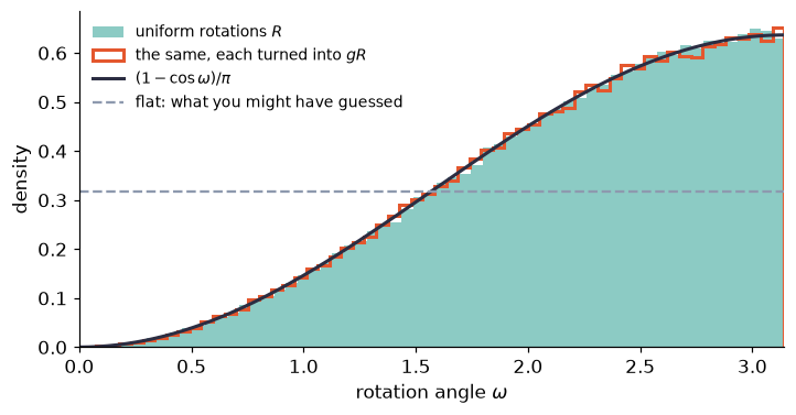
Recap. A uniform distribution on a group is one that multiplying by a fixed element leaves unchanged. It exists (and is unique) exactly for compact groups: finite groups, the circle, rotations. It does not exist for . "Uniform" is a statement about the group, not about any coordinate, so a uniform rotation does not have a uniform angle.
Check yourself
- Show from the definition that the uniform distribution on must give every element probability .
Answer
Take (adding 1). Invariance says for every , so all elements have the same probability. The probabilities sum to 1, so each is .
- Why can't there be a uniform distribution on (with multiplication)?
Answer
Invariance under multiplying by 2 would force the intervals (and ) to all have the same probability. There are infinitely many of these disjoint intervals, so that common probability must be 0. But they cover all of , so the total would be 0, not 1.
- Here is a recipe for a random rotation: pick a uniformly random axis and an angle uniform in . Is the result uniform on ?
Answer
No. Its angle histogram would be the flat dashed line, not , so it gives far too many small rotations.
2. Putting a price on defects: face cost and total cost
Now the tilt. We want labelings with defects to be less likely, and big defects even less likely than small ones. So we first attach a price to every face.
Definition (face cost, glossary 4.2). A face
cost is a function
that is a class function, so
,
and that is smallest at the identity. We use the standard choice,
written in lgt as standard_face_cost(G):
| group | face cost |
|---|---|
| coin | |
| circle , and drawn as angles | |
| matrices ( as permutation matrices, ) |
Definition (total cost, glossary 4.3). For a board with faces , the total cost of a labeling is
For the coin group, .
The plot shows the face cost on the circle, with the elements of and sitting on the same curve. is a finite "pixelation" of the circle.
th = np.linspace(0, 2 * np.pi, 400)
fig, ax = plt.subplots(figsize=(7, 3.2))
ax.plot(th, standard_face_cost(U1())(th), color=viz.INK, lw=2, label=r"circle: $\varphi(\theta)=1-\cos\theta$")
for G, mk, ms in [(ZN(5), "s", 8), (Z2(), "o", 15)]:
    x = G.elements()
    ax.plot(G.angle(x), standard_face_cost(G)(x), mk, ms=ms, mfc="none", mew=2.5,
            label=f"elements of {G}")
ax.set(xlabel=r"face product, as an angle $\theta$", ylabel=r"$\varphi$",
       xticks=[0, np.pi, 2 * np.pi], xticklabels=["0", r"$\pi$", r"$2\pi$"])
ax.legend(frameon=False, fontsize=9)
plt.show()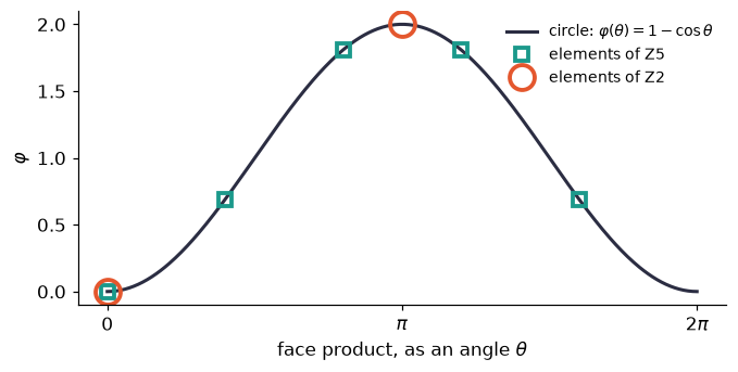
Why do we insist that is a class function? A face product depends on where you start walking around the face, and on the reframing. Both change it only by a conjugation (glossary 3.5). A class function doesn't notice either.
Fact 2.3 (total cost is an invariant). For every labeling and every reframing , .
Let's check it on a grid with four groups: finite and continuous, abelian and non-abelian.
B = Board.grid(4, 4)
for G in [Z2(), U1(), S3(), SO3()]:
    M = Model(B, G)
    U, h = random_labeling(G, B, rng), random_reframing(G, B, rng)
    print(f"{str(G):>4}:  S(U) = {M.cost(U):8.4f}   S(reframed U) = {M.cost(reframe(G, B, U, h)):8.4f}")
Z2: S(U) = 10.0000 S(reframed U) = 10.0000
U1: S(U) = 9.5657 S(reframed U) = 9.5657
S3: S(U) = 12.0000 S(reframed U) = 12.0000
SO3: S(U) = 23.7503 S(reframed U) = 23.7503
Here is one random coin labeling on that grid. Gold edges carry , coral faces are defects. Count the coral faces and double the count: that's .
G, B = Z2(), Board.grid(4, 4)
U = random_labeling(G, B, rng)
fig, ax = plt.subplots(figsize=(4, 4))
viz.draw_board(ax, B, U, G, title=f"S(U) = {Model(B, G).cost(U):.0f}  "
               f"({defects(G, B, U).sum()} defects)")
plt.show()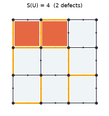
Recap. A face cost prices a single face. It is a class function, minimal at the identity. The total cost adds up the prices of all faces. Because ignores conjugation, is an invariant: reframings don't change it.
Check yourself
- A coin-group labeling on the grid has 3 defects. What is ?
Answer
.
- A face is a closed walk, but which vertex does it start at? Explain why this choice cannot affect .
Answer
Starting the same loop at a different vertex turns the product into, for example, . That is a conjugate, and a class function gives conjugates the same value.
- On the circle, for which face products is the face cost zero?
Answer
Only for , the identity. for every other angle.
3. Stiffness and the model
One more ingredient: a single number that says how seriously to take the cost.
Definition (stiffness, glossary 4.4). The stiffness is a number. Large means defects are heavily punished; means cost is ignored.
Definition (model, glossary 4.5). Let be "every edge label uniform and independent", a probability distribution on . The model with board , group , face cost and stiffness is the probability distribution on given by
For a finite group, the integral is just an average over the labelings, and this reads
is just the normalizing number that makes the probabilities add up to 1.
The stance of this course. The model is the object we study. The cost is not extra information on top of it. Up to the constant , the scaled cost is just minus the logarithm of the density of relative to uniform:
So a model is completely specified by four things: (board, , , ).
For finite groups, lgt computes
exactly, by listing every labeling. Let's do that for the coin
model on the
torus from the opening puzzle:
labelings.
T = Board.grid(2, 2, periodic=True)
beta = 1.0
ex = Model(T, Z2(), beta=beta).exact()          # every labeling with its probability
k = (ex.cost / 2).astype(int)                   # number of defects of each labeling
for kk in np.unique(k):
    sel = k == kk
    print(f"{kk} defects: {sel.sum():3d} labelings, each with probability "
          f"{ex.p[sel][0]:.5f}  (together {ex.p[sel].sum():.3f})")
print(f"\nZ(beta={beta}) = {np.exp(ex.log_Z):.5f}")
print("cost = log-density?", np.allclose(-np.log(ex.p * 256), beta * ex.cost + ex.log_Z))
0 defects: 32 labelings, each with probability 0.02815 (together 0.901)
2 defects: 192 labelings, each with probability 0.00052 (together 0.099)
4 defects: 32 labelings, each with probability 0.00001 (together 0.000)
Z(beta=1.0) = 0.13878
cost = log-density? True
Three things to notice:
- A torus never has exactly 1 or 3 defects. Every edge lies on exactly two faces, so the product of all face products is always . We'll come back to this in section 5.
- Each individual 4-defect labeling is times as likely as a 0-defect labeling.
- The last line confirms the stance: of the density is .
And the opening puzzle: with fair coins (), each face is a defect with probability , so you expect defects out of 4.
Recap. A model is the uniform distribution on labelings, reweighted by and renormalized by . It is determined by (board, , , ). Up to sign, scale and a constant, the cost is the log-density relative to uniform, so the model is the single object that holds everything.
Check yourself
- In the torus model at , how much less likely is a particular labeling with 2 defects than a particular labeling with none?
Answer
The costs are and , so the ratio is . The normalizer cancels in ratios.
- Someone hands you as a table of probabilities but forgets to tell you . Can you recover ?
Answer
Yes, up to an additive constant: . The constant is pinned down by the identity labeling, whose cost is 0.
- What happens to the model if you double and halve ?
Answer
Nothing. Only the product enters . Stiffness is the convention for "how sharp" the cost is, measured against a fixed .
4. Redundancy does no harm
In chapter 1 we saw that a labeling carries both real information (its class) and convention (a reframing). Does that convention distort the model? No, for three reasons.
Fact 2.4 (the model doesn't see reframings). For every reframing and every labeling : . Equivalently, reframing a random labeling drawn from gives a random labeling with the same distribution .
Why: a reframing permutes the labelings, it leaves unchanged, and it leaves unchanged (Fact 2.3). Below we reframe all 256 labelings at once, see where each one lands, and compare probabilities.
def index_of(U):
    """Position of a coin labeling in the enumeration order of `Model.exact()`."""
    bits = (np.asarray(U) == -1).astype(np.int64)
    return bits @ (2 ** np.arange(bits.shape[-1])[::-1])

assert np.all(index_of(ex.U) == np.arange(len(ex.U)))
h = random_reframing(Z2(), T, rng)
moved = index_of(reframe(Z2(), T, ex.U, h))           # where each labeling goes
print("reframing permutes the labelings:", len(np.unique(moved)) == len(moved))
print("and preserves every probability: ", np.allclose(ex.p[moved], ex.p))
reframing permutes the labelings: True
and preserves every probability: True
Next, how big are the classes? For an abelian group they all have the same size.
Fact 2.5 (class sizes). If is finite and abelian (recall that boards are connected), every class contains exactly labelings, and there are classes. Hence the probability of a class is proportional to of any of its members.
For non-abelian , classes can have different sizes.
Why the exponent is : there are reframings. When is abelian, a reframing leaves a labeling unchanged exactly when on every edge, that is, when is constant. So each labeling in a class is reached by exactly reframings, and the class has members.
sizes = np.bincount(class_ids(Z2(), T, ex.U))
print(f"coin on the torus: {len(sizes)} classes, sizes {set(sizes.tolist())}"
      f"  (formula: 2^{T.cycle_rank} classes of size 2^{T.n_vertices - 1})")

S, tri = S3(), Board.triangle()
Us = all_labelings(S, tri)
ids = class_ids(S, tri, Us)
loop = loop_product(S, tri, Us, [0, 1, 2, 0])
for c in range(ids.max() + 1):
    print(f"S3 on the triangle, class {c}: {np.sum(ids == c):3d} labelings, "
          f"loop product like {viz.format_label(S, loop[ids == c][0])}")
coin on the torus: 32 classes, sizes {8} (formula: 2^5 classes of size 2^3)
S3 on the triangle, class 0: 36 labelings, loop product like e
S3 on the triangle, class 1: 108 labelings, loop product like (23)
S3 on the triangle, class 2: 72 labelings, loop product like (123)
On the triangle with , a class is determined by the conjugacy class of its loop product (chapter 1). The 216 labelings split , because identity, transpositions and 3-cycles make up , and of . So, unlike the abelian case, the class sizes differ. That's fine: the size is simply how much uniform probability the class carries.
The most useful form of "redundancy does no harm" is the next fact. It lets us throw the redundancy away before computing. It is about averages: for a function , we write for its expectation when is drawn from (glossary 4.6). Chapter 3 is all about averages; here we only need the notation.
Fact 2.6 (fixing the tree is free). Pick a spanning tree. For any invariant , the average equals the average of in the smaller model where every tree edge is fixed to the identity and only the other labels are random (with the same weight ).
Why: putting a uniformly random labeling into tree normal form leaves the non-tree labels uniform and independent. Each of them is a walk product that contains its own edge's uniform label exactly once. Invariants and don't change.
Let's verify this with two invariants on the torus (the number of defects, and the face product of one face) and one on the triangle ( of the loop product, where is the trace of the permutation matrix).
def tree_fixed_average(model, f):
    """Average of f when tree labels are pinned to the identity (Fact 2.6)."""
    tree = model.board.spanning_tree()[0]
    ex = model.exact()
    keep = np.all(model.G.is_identity(ex.U[:, tree]), axis=1)
    p = ex.p[keep] / ex.p[keep].sum()
    return float(np.sum(p * f(ex.U[keep]))), int(keep.sum())

M = Model(T, Z2(), beta=0.7)
for name, f in [("number of defects", lambda U: defects(Z2(), T, U).sum(-1)),
                ("product of face 0", lambda U: face_products(Z2(), T, U)[:, 0])]:
    small, n = tree_fixed_average(M, f)
    print(f"{name:>25}: full model {M.average(f):+.5f} | tree fixed {small:+.5f} ({n} labelings)")

Mt = Model(tri, S, beta=0.7)
chi = lambda U: S.chi(loop_product(S, tri, U, [0, 1, 2, 0]))
print(f"{'S3 triangle, chi(loop)':>25}: full model {Mt.average(chi):+.5f} | "
      f"tree fixed {tree_fixed_average(Mt, chi)[0]:+.5f}")
number of defects: full model +0.54401 | tree fixed +0.54401 (32 labelings)
product of face 0: full model +0.72799 | tree fixed +0.72799 (32 labelings)
S3 triangle, chi(loop): full model +1.88431 | tree fixed +1.88431
Same numbers, from instead of labelings on the torus, and from 6 instead of 216 on the triangle. On big boards this saving is enormous.
Recap. Reframings permute labelings without changing their probability (Fact 2.4). For abelian groups all classes have the same size, so the redundancy is a constant overcount that cancels (Fact 2.5). For any group, you may pin a spanning tree to the identity before computing averages of invariants (Fact 2.6).
Check yourself
- Coin model on the torus (9 vertices, 18 edges). How many classes, and how big is each?
Answer
classes, each with labelings. Check: .
- With on the triangle, the class of the identity labeling has only 36 members. Which reframings leave the identity labeling unchanged?
Answer
The six constant reframings : they give on every edge. Each labeling in the class is therefore produced by 6 different reframings, and the reframings give only different labelings. A labeling whose loop product is a 3-cycle is fixed by only 3 reframings, so its class has members.
- Fact 2.6 needs to be an invariant. Find a non-invariant for which it fails.
Answer
In the coin model, take for a tree edge . In the tree-fixed model it is always , so its average there is . In the full model its average is , as chapter 3 explains.
5. The stiffness dial
What does turning do? Look at the two ends first.
Fact 2.7 (the two ends of the dial).
- At , : all labels are independent and uniform.
- As , piles up on the labelings with no defects (cost 0), spread uniformly over them.
On a torus, "no defects" is a weaker condition than "consistent" (glossary 2.6). A loop that goes once around the torus is not a product of faces, so its loop product can still be when every face product is . On the torus there are 32 defect-free labelings, but only 8 consistent ones.
for beta in [0.0, 1.0, 3.0, 6.0]:
    ex_b = Model(T, Z2(), beta=beta).exact()
    k = (ex_b.cost / 2).astype(int)
    ok = is_consistent(Z2(), T, ex_b.U)
    print(f"beta = {beta:3.1f}:  P(no defects) = {ex_b.p[k == 0].sum():.4f}   "
          f"P(consistent) = {ex_b.p[ok].sum():.4f}")
print("defect-free labelings:", int(np.sum(k == 0)), "| consistent:", int(ok.sum()))
beta = 0.0: P(no defects) = 0.1250 P(consistent) = 0.0312
beta = 1.0: P(no defects) = 0.9007 P(consistent) = 0.2252
beta = 3.0: P(no defects) = 1.0000 P(consistent) = 0.2500
beta = 6.0: P(no defects) = 1.0000 P(consistent) = 0.2500
defect-free labelings: 32 | consistent: 8
At large , settles at : the model spreads evenly over the 32 defect-free labelings, and only 8 of them are consistent.
Now the whole dial, on the torus ( labelings, still exact). The weight of a labeling depends only on its number of defects . So we count the labelings with each once, at , and reweight: , where is that count.
What to look at:
- Left: at the defect count is a binomial-like hump around half the faces (only even counts are possible, as before). As grows the hump slides to 0.
- Right: the average fraction of defect faces drops smoothly. The dashed curve is a formula for planar grids (not wrapped around), coming next.
T3 = Board.grid(3, 3, periodic=True)
ex3 = Model(T3, Z2(), beta=0.0).exact()
N_k = np.bincount((ex3.cost / 2).astype(int))           # labelings with k defects
kk = np.arange(len(N_k))
def P_defects(beta):
    w = N_k * np.exp(-2 * beta * kk)
    return w / w.sum()

betas = np.linspace(0, 2.5, 101)
mean_frac = [P_defects(b) @ kk / T3.n_faces for b in betas]
fig, (a1, a2) = plt.subplots(1, 2, figsize=(11, 3.6))
for i, b in enumerate([0, 0.3, 0.6, 1.0, 2.0]):
    a1.bar(kk + (i - 2) * 0.16, P_defects(b), width=0.16, label=fr"$\beta={b}$")
a1.set(xlabel="number of defects $k$ (of 9 faces)", ylabel="probability", xticks=kk)
a1.legend(frameon=False, fontsize=9)
a2.plot(betas, mean_frac, lw=2.5, label=r"$3\times3$ torus (exact)")
a2.plot(betas, np.exp(-2 * betas) / (1 + np.exp(-2 * betas)), "--", color=viz.INK,
        label=r"planar grid: $e^{-2\beta}/(1+e^{-2\beta})$")
a2.set(xlabel=r"stiffness $\beta$", ylabel="average fraction of defect faces")
a2.legend(frameon=False, fontsize=9)
plt.show()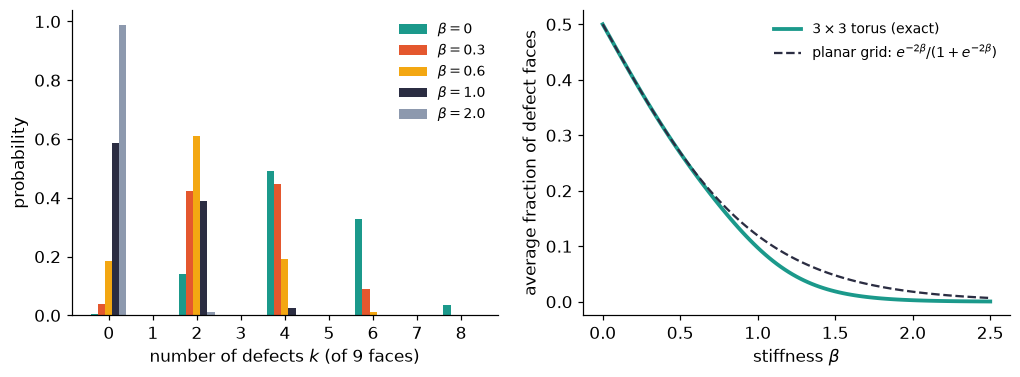
On a planar grid, the faces are independent coins
The dashed curve comes from a fact that makes the coin model on a planar grid almost embarrassingly simple. Chapter 3 builds on it.
Fact 2.8 (independent faces). In the coin model (, standard face cost) on a planar grid (not wrapped around), the face products , one per face , are independent. Each is a defect with probability ; equivalently, .
Why, lightly: put the labeling in tree normal form (Fact 2.6). On a planar grid the number of non-tree edges equals the number of faces, since for an grid. The non-tree labels and the face products determine each other one-to-one. So the face products are independent fair coins under . The weight then tilts each coin separately.
Let's check it exactly on the grid (12 edges, 4 faces). We compare all 16 joint probabilities of the four face products with the product of the four marginals.
P3 = Board.grid(3, 3)
beta = 0.6
exP = Model(P3, Z2(), beta=beta).exact()
FP = face_products(Z2(), P3, exP.U)                      # (4096, 4): one row per labeling
patterns = np.array(np.meshgrid(*[[1, -1]] * 4, indexing="ij")).reshape(4, -1).T
marg = (1 + np.tanh(beta) * patterns) / 2                # P(U_f = s) = (1 + s tanh beta)/2
joint = np.array([exP.p[np.all(FP == s, axis=1)].sum() for s in patterns])
print("largest |joint - product of marginals| over 16 patterns:",
      f"{np.abs(joint - marg.prod(axis=1)).max():.1e}")
print(f"<U_f> = {exP.average(lambda U: face_products(Z2(), P3, U)[:, 0]):.5f}"
      f"   tanh(beta) = {np.tanh(beta):.5f}")
largest |joint - product of marginals| over 16 patterns: 5.6e-17
<U_f> = 0.53705 tanh(beta) = 0.53705
The independence fails on a torus, and we already know why: there the product of all face products is forced to be .
FP3 = face_products(Z2(), T3, ex3.U)
print("3x3 torus: product of all face products is +1 for every labeling:",
      bool(np.all(FP3.prod(axis=1) == 1)))
3x3 torus: product of all face products is +1 for every labeling: True
Seeing the dial
Fact 2.8 hands us an exact sampler for large planar grids, far too large to enumerate. Flip one tilted coin per face. Then build any labeling with those face products: keep vertical edges at and fill in the horizontal edges row by row. Finally apply a random reframing so that the labeling doesn't look special. (By Fact 2.4 the result is an exact draw from .)
What to look at:
- The faces: the coral defects thin out as grows.
- The edges: the gold edges look like the same random noise at every .
Edge labels are mostly convention. The information lives on the faces.
def sample_coin_planar(L, beta, rng):
    """Exact draw from the coin model on an L x L planar grid (Fact 2.8 + Fact 2.4)."""
    B, G = Board.grid(L, L), Z2()
    idx = B.meta["edge_index"]                           # (vertex, direction) -> edge
    p = np.exp(-2 * beta) / (1 + np.exp(-2 * beta))
    face = np.where(rng.random((L - 1, L - 1)) < p, -1, 1)
    U = G.identity(B.n_edges)                            # vertical edges stay +1
    for y in range(L - 1):
        for x in range(L - 1):                           # face (x,y) = bottom edge * top edge
            U[idx[(x + L * (y + 1), 0)]] = U[idx[(x + L * y, 0)]] * face[x, y]
    return B, reframe(G, B, U, random_reframing(G, B, rng))
fig, axs = plt.subplots(1, 4, figsize=(16, 4.4))
for ax, beta in zip(axs, [0.0, 0.5, 1.0, 2.0]):
B, U = sample_coin_planar(10, beta, rng)
viz.draw_board(ax, B, U, Z2(), show_arrows=False, vertex_size=8, pad=0.2,
title=fr"$\beta={beta}$: {defects(Z2(), B, U).sum()} defects of {B.n_faces}")
plt.show()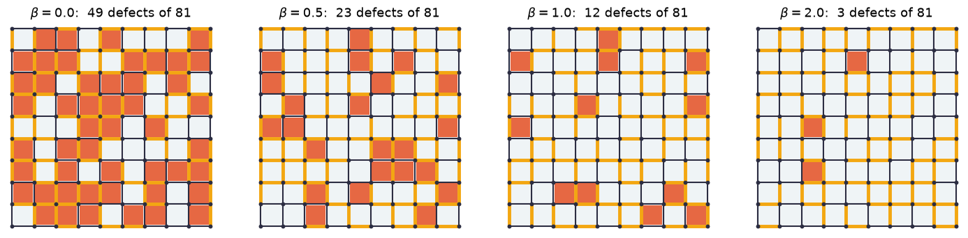
The same dial works for any compact group. Here is the circle on a grid. The samples come from a simple random-update sampler, which we'll explain in chapter 4. Clock hands show the edge labels, and face colour shows the face product as an angle: pale means near the identity, dark means far from it. Again the clock hands look random at every stiffness, while the faces calm down.
G, B = U1(), Board.grid(6, 6)
fig, axs = plt.subplots(1, 4, figsize=(16, 4.4))
for ax, beta in zip(axs, [0.0, 1.0, 3.0, 10.0]):
    step = min(1.0, 1.5 / np.sqrt(beta + 1e-9))          # smaller moves when stiff
    U = Model(B, G, beta=beta).metropolis(rng, n_samples=1, burn_in=400, step=step)[0]
    viz.draw_board(ax, B, U, G, show_arrows=False, vertex_size=8, clock_r=0.13,
                   title=fr"$\beta={beta}$")
plt.show()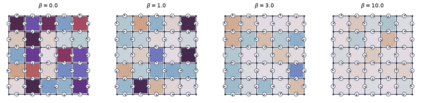
Recap. At the model is uniform, and as it piles up on the defect-free labelings. On a torus those include non-consistent ones, whose loop product once around the torus is not the identity. On a planar grid with the coin group, the faces are independent coins with (Fact 2.8). Pictures of samples show the lesson of this chapter: edges look like noise, and faces carry the information.
Check yourself
- In the planar-grid coin model, what is the probability that a given face is a defect at ? At ?
Answer
At it is . At , , so the probability is .
- Why can a torus never have exactly one defect?
Answer
Every edge lies on exactly two faces. In the product of all face products, each label appears twice, and . So the product of all face products is , which means the number of defects is even.
- The grid in the dial picture has edges. How many labelings is that, and why could we still sample it exactly?
Answer
labelings, far beyond enumeration. Fact 2.8 reduces the problem to 81 independent tilted coins, one per face. Fact 2.4 lets us reframe the result freely.
Chapter recap
- A uniform distribution on is unchanged by multiplying by a fixed element. It exists exactly for compact (finite groups, circle, rotations), not for . A uniform rotation's angle has density .
- A face cost is a class function, minimal at the identity. The total cost is an invariant.
- The model is determined by (board, , , ). The cost is its log-density relative to uniform, so the model is the one object that holds everything.
- Redundancy does no harm: reframings preserve . Abelian classes all have size . You may pin a spanning tree to the identity before averaging invariants.
- The stiffness dial runs from uniform labels () to defect-free labelings ().
- On a planar grid with the coin group, faces are independent coins with .
Dictionary
| Our term | Other names |
|---|---|
| uniform distribution on | Haar measure |
| face cost | Wilson action (per plaquette) |
| total cost | action, Euclidean action; energy (statistical mechanics) |
| stiffness | inverse coupling (up to a constant); inverse temperature |
| model | lattice gauge theory; "the theory"; Euclidean path integral; Gibbs measure |
| normalizer | partition function |
| average | expectation value; vacuum expectation value |
| coin model | lattice gauge theory (Wegner's Ising gauge model) |
| fixing the tree (Fact 2.6) | gauge fixing (maximal-tree / axial gauge) |
What's next
A model is a distribution, but we can only ever ask it questions: "on average, what is this number?" Chapter 3 is about which questions make sense. Averages of non-invariant quantities, like a single edge label, turn out to be useless, and you'll see exactly why. Averages of loop products are where the structure shows up. On a planar grid, Fact 2.8 already tells you how the average loop product of a big rectangle must behave. Try to guess before you turn the page.