← Eyal Merhavi · Labelings, models, and gauge theory
Chapter 3 of Labelings, models, and gauge theory, rendered from the executed notebook. Code cells and their outputs are shown as they ran.
Run this chapter in your browser ↗ · Source on GitHub ↗
Runs on JupyterLite. The first time, it downloads Python and its libraries (about 40 MB).
Chapter 3: What a model can tell you
In Chapter 2 you built a model: a probability distribution on the labelings of a board. A model answers questions, and this chapter is about which questions are worth asking.
Here is a puzzle to start. Take the coin model () on a small grid and turn the stiffness up to . Now almost every face is calm (not a defect): each face product is with probability . The board looks frozen. Surely the edge labels have "settled" on some values? So here is the question: what is the average label on one edge? Make a guess before you scroll down.
What you'll learn
- How to ask a model a question: the average of a quantity .
- Why a single edge label averages to exactly zero at every stiffness, and why this means a model only ever "knows" invariants.
- How loop observables behave on a grid (they decay with area), and why loop observables are enough to pin down a class.
Prerequisites:
- Chapter 1: labelings, walk and loop products, reframings, classes, invariants, class functions, loop observables.
- Chapter 2: face cost, total cost, stiffness, models, exact enumeration.
import numpy as np
import matplotlib as mpl
import matplotlib.pyplot as plt
from IPython.display import HTML

from lgt import *
from lgt import viz

viz.use_style()
rng = np.random.default_rng(2026)
1. Asking a model a question: averages
A model is a probability distribution on labelings. A question is any function of the labeling, and the model answers it with an average.
Definition (average, glossary 4.6). Take a model on a board with label group . A quantity is any function . Its average is the number
For a continuous group like the circle, the sum becomes an integral against . Recall from Chapter 2 that for finite :
The map is linear: .
Example. Take the coin model on a
grid of vertices, which has 12 edges and 4 faces. It has
labelings, few enough to list them all. Model.exact() does
exactly that, and .average(f) computes the weighted sum. We
ask two questions:
- What is the total cost on average?
- What is the face product of the bottom-left face on average?
B = Board.grid(3, 3)
G = Z2()
print(B)
print(" beta   <S>      <U_f>    tanh(beta)")
for beta in [0.0, 0.5, 1.0, 2.0]:
    M = Model(B, G, beta)
    ex = M.exact()                                  # all 4096 labelings and their probabilities
    avg_S = ex.average(M.cost)
    avg_face = ex.average(lambda U: face_products(G, B, U)[:, 0])
    print(f"{beta:5.1f}  {avg_S:6.3f}  {avg_face:8.4f}  {np.tanh(beta):8.4f}")
Board('3x3 grid': 9 vertices, 12 edges, 4 faces)
beta <S> <U_f> tanh(beta)
0.0 4.000 0.0000 0.0000
0.5 2.152 0.4621 0.4621
1.0 0.954 0.7616 0.7616
2.0 0.144 0.9640 0.9640
What to look at:
- As grows, the average cost falls and faces become calm.
- The average face product matches , as Chapter 2 predicted for planar grids.
Recap. A question to a model is a quantity . The answer is the average , and averaging is linear in .
Check yourself
- At , what is for the coin model on this board?
Answer
At , every labeling is equally likely, so each face product is with probability . The face cost is and , so each face costs on average. With 4 faces, , which matches the table.
- What is , the average of the constant function ?
Answer
It is , because the probabilities sum to one.
2. The edge never decides
Back to the puzzle. Pick the edge from vertex 0 to vertex 1, and compute its average label exactly, next to the average face product.
e = 0
print("edge", e, "goes from vertex", B.edges[e][0], "to vertex", B.edges[e][1])
print(" beta     <U(e)>      <U_f>")
for beta in [0.0, 1.0, 2.0, 5.0]:
    ex = Model(B, G, beta).exact()
    edge_avg = round(ex.average(lambda U: U[:, e]), 9) + 0.0
    face_avg = ex.average(lambda U: face_products(G, B, U)[:, 0])
    print(f"{beta:5.1f}   {edge_avg:+.6f}   {face_avg:.6f}")
edge 0 goes from vertex 0 to vertex 1
beta <U(e)> <U_f>
0.0 +0.000000 0.000000
1.0 +0.000000 0.761594
2.0 +0.000000 0.964028
5.0 +0.000000 0.999909
The edge average is exactly zero at every stiffness, even at where the faces are almost perfectly calm. Here is the whole distribution at .
- The left panel shows one typical labeling drawn from the model. Gold edges () are scattered everywhere, yet every face is calm (pale).
- The right panel compares the distribution of the edge label with that of a face product.
beta = 3.0
ex = Model(B, G, beta).exact()
U_draw = ex.sample(rng, 1)[0]
p_edge = [ex.average(lambda U: U[:, e] == s) for s in (1, -1)]
p_face = [ex.average(lambda U: face_products(G, B, U)[:, 0] == s) for s in (1, -1)]

fig, (a0, a1) = plt.subplots(1, 2, figsize=(10.5, 4.2), gridspec_kw=dict(width_ratios=[1, 1.3]))
viz.draw_board(a0, B, U_draw, G, edge_labels={e: "e"}, title=f"one labeling drawn at β = {beta:g}")
a0.text(*B.face_polys[0].mean(axis=0)[:2], "f", ha="center", va="center", fontsize=13, color=viz.INK)
vals = p_edge + p_face
a1.bar(range(4), vals, color=[viz.TEAL, viz.TEAL, viz.CORAL, viz.CORAL])
for i, v in enumerate(vals):
    a1.text(i, v + 0.02, f"{v:.4f}", ha="center")
a1.set_xticks(range(4), ["$U(e)=+1$", "$U(e)=-1$", "$U_f=+1$", "$U_f=-1$"])
a1.set_ylim(0, 1.12); a1.set_ylabel("probability under $\\mu_\\beta$")
a1.set_title("the edge is a fair coin; the face is not")
plt.show()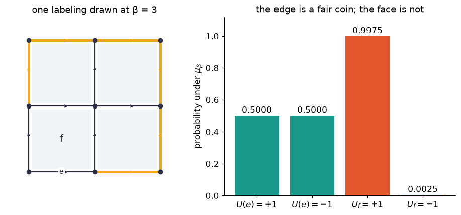
The same thing happens with circle labels (, labels are angles), where the effect is even easier to see.
- The model is now too big to enumerate, so we use a sampler: an algorithm that produces labelings distributed approximately according to . Chapter 4 opens this black box.
- We start the sampler from the labeling with every angle equal to , so every edge starts out "decided".
- We use stiffness on a grid.
GU, BU = U1(), Board.grid(4, 4)
start = identity_labeling(GU, BU)                       # every edge starts at angle 0
samples = Model(BU, GU, beta=4.0).metropolis(rng, 4000, sweeps_between=4, burn_in=300,
                                             U0=start, step=0.5)
eU = BU.meta["edge_index"][(5, 0)]                      # an interior edge, leaving vertex (1,1)
fU = [c for c, mu, nu in BU.meta["face_anchor"]].index((1, 1))   # the face anchored at (1,1)
edge_angles, face_angles = samples[:, eU], face_products(GU, BU, samples)[:, fU]
print("edge: <cos U(e)> = %+.3f   <sin U(e)> = %+.3f" % (np.cos(edge_angles).mean(), np.sin(edge_angles).mean()))
print("face: <cos U_f>  = %+.3f   <sin U_f>  = %+.3f" % (np.cos(face_angles).mean(), np.sin(face_angles).mean()))
edge: <cos U(e)> = -0.020 <sin U(e)> = +0.011
face: <cos U_f> = +0.862 <sin U_f> = +0.008
Below, the left panel is the last labeling the sampler produced. The clock hands point in every direction, yet every face is only lightly tinted: each face product is close to angle , which is drawn as white, and blue and brown tints mean small turns one way or the other. The two dials on the right are histograms around the circle: how often each angle occurs.
- For the edge, the histogram is flat. It matches the dashed circle, which is the uniform distribution.
- For the face, the histogram is a spike at angle .
fig = plt.figure(figsize=(14, 4.6))
viz.draw_board(fig.add_subplot(1, 3, 1), BU, samples[-1], GU, title="a late sample (β = 4)")
for k, (vals, name, col) in enumerate([(edge_angles, "edge label $U(e)$", viz.TEAL),
                                       (face_angles, "face product $U_f$", viz.CORAL)]):
    ax = fig.add_subplot(1, 3, k + 2, projection="polar")
    ax.set_thetagrids([0, 90, 180, 270], ["0", "π/2", "π", "3π/2"])
    dens, bins = np.histogram(vals, bins=36, range=(0, 2 * np.pi), density=True)
    ax.bar(bins[:-1], dens, width=bins[1] - bins[0], align="edge", color=col, alpha=0.85)
    th = np.linspace(0, 2 * np.pi, 200)
    ax.plot(th, np.full_like(th, 1 / (2 * np.pi)), "--", color=viz.INK, lw=1)
    ax.set_yticklabels([]); ax.set_title(name, pad=14)
plt.show()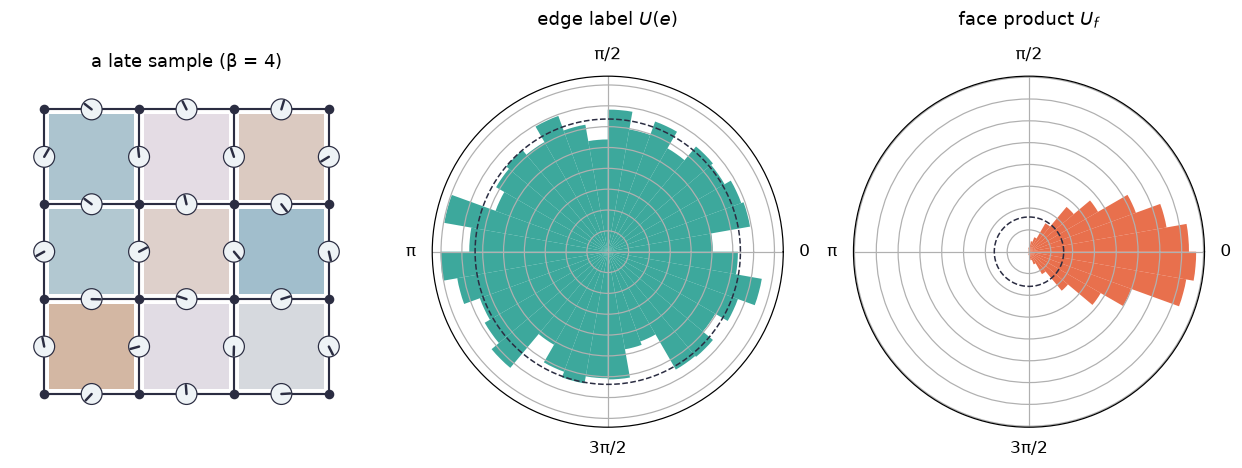
Fact 3.1 (single-edge labels are uniform). Take any model: any board, any compact label group , any face cost, any stiffness . For every edge whose two endpoints are different, the label is uniformly distributed on . In particular:
- for the coin model;
- for circle labels.
Why. Write as and pick any . Use the reframing with and at every other vertex.
- It changes to .
- It leaves unchanged. The total cost is an invariant, and the uniform distribution doesn't change when labels are multiplied by .
So and have the same distribution, for every . The only distribution on that is unchanged by every multiplication is the uniform one.
So high stiffness calms the faces, but it says nothing about individual edges. Every reframing of the all-identity labeling has no defects, so they all cost the same, and the model spreads its probability evenly over all of them.
Recap. A quantity that a reframing can change, like a single edge label, gets smeared out by the model. Its distribution is uniform at every , so its average carries no information.
Check yourself
- In a model with (permutations of three things), what is the probability that ?
Answer
It is , the same as for every other element, at every (Fact 3.1).
- Take an open walk from to with . Is its walk product uniform too?
Answer
Yes. A reframing at alone multiplies on the left by , because the inner factors cancel (Chapter 1). Only closed walks escape this argument, because their two ends are the same vertex.
- Why did the fact need the endpoints of to be different?
Answer
If goes from back to , a reframing changes its label to , a conjugate. Its conjugacy class can't be changed this way, so its label need not be uniform. Such an edge is itself a closed walk.
3. What a model really knows: a distribution on classes
Fact 3.1 is one instance of a general rule: averaging over reframings never changes an average.
Fact 3.2 (averages only see invariants). For a quantity , define its reframing average by letting be the average of over a uniformly random reframing . For finite this is . Then is an invariant, and for every .
Why. Every reframing leaves unchanged, so replacing by doesn't change its average. Averaging over all reframings doesn't change it either.
We check this on the coin model on the torus, which has 4 vertices, 8 edges and 4 faces. The quantity is deliberately not an invariant: "edge 0 is and face 0 is calm."
T = Board.grid(2, 2, periodic=True)
exT = Model(T, G, beta=1.0).exact()
H = all_reframings(G, T)                                    # all 2^4 = 16 reframings

def f(U):           # not an invariant
    return ((U[..., 0] == 1) & (face_products(G, T, U)[..., 0] == 1)).astype(float)

def f_bar(U):       # its reframing average
    return np.mean([f(reframe(G, T, U, h)) for h in H], axis=0)

print("<f> =", round(exT.average(f), 6), "   <f_bar> =", round(exT.average(f_bar), 6))
print("f_bar is an invariant:", all(np.allclose(f_bar(exT.U), f_bar(reframe(G, T, exT.U, h))) for h in H))
print("f is an invariant:    ", all(np.allclose(f(exT.U), f(reframe(G, T, exT.U, h))) for h in H))
<f> = 0.475103 <f_bar> = 0.475103
f_bar is an invariant: True
f is an invariant: False
So everything a model can tell you comes from the probabilities it gives to classes. Each class has the same number of members (Chapter 2), so the probability of a class is proportional to .
On this small board there are labelings, which fall into classes. The chart below shows the probability of each of the 32 classes at two stiffnesses. Each bar is coloured by how many defects the class has.
ids = class_ids(G, T, exT.U)                       # class of each of the 256 labelings
first = np.unique(ids, return_index=True)[1]       # one representative per class
cls_def = defects(G, T, exT.U).sum(axis=1)[first]  # number of defects in each class
colors = {0: viz.TEAL, 2: viz.GOLD, 4: viz.CORAL}
print(len(exT.U), "labelings,", len(first), "classes, sizes:", set(np.bincount(ids)))

fig, axes = plt.subplots(1, 2, figsize=(11.5, 3.6), sharey=True)
for ax, beta in zip(axes, [0.5, 2.0]):
    p = np.bincount(ids, weights=Model(T, G, beta).exact().p)
    order = np.argsort(-p, kind="stable")
    ax.bar(range(len(p)), p[order], color=[colors[d] for d in cls_def[order]])
    ax.set_title(f"β = {beta:g}"); ax.set_xlabel("the 32 classes, most likely first")
axes[0].set_ylabel("probability of the class")
axes[1].legend([plt.Rectangle((0, 0), 1, 1, color=c) for c in colors.values()],
               [f"{d} defects" for d in colors], frameon=False)
plt.show()
256 labelings, 32 classes, sizes: {np.int64(8)}
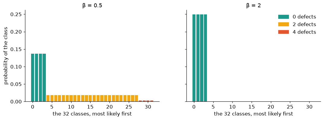
At high stiffness, nearly all the probability sits on four classes with no defects, tied with each other. Why four? On a board that wraps around, some loops aren't built out of faces:
- the loop that goes once around horizontally;
- the loop that goes once around vertically.
Their loop products are invariants that the faces can't see.
Below are the four calm classes, each drawn in tree normal form (the spanning tree is in grey). To draw a board that wraps around, we unroll it: the right column of dots is the same as the left column, and the top row is the same as the bottom row. Those copies are drawn as hollow dots, and the copied edges repeat the labels.
- The loop "around x" is the bottom row of edges.
- The loop "around y" is the left column.
Every face is pale, and the four classes differ only in those two loops.
eT = T.meta["edge_index"]
around_x = [(eT[(0, 0)], 1), (eT[(1, 0)], 1)]      # 0 -> 1 -> back to 0 (wrapping)
around_y = [(eT[(0, 1)], 1), (eT[(2, 1)], 1)]      # 0 -> 2 -> back to 0 (wrapping)
flat = Board.grid(3, 3)                            # the unrolled picture of the 2x2 torus

def unroll(U_T):
    """Copy labels of the 2x2 torus onto the unrolled 3x3 picture."""
    to_T = {e: eT[((x % 2) + 2 * (y % 2), mu)]
            for (v, mu), e in flat.meta["edge_index"].items() for x, y in [flat.meta["coord"][v]]}
    return np.array([U_T[to_T[e]] for e in range(flat.n_edges)]), to_T

fig, axes = plt.subplots(1, 4, figsize=(13, 3.6))
for ax, c in zip(axes, [c for c in range(len(first)) if cls_def[c] == 0]):
    Un, _, tree = tree_normal_form(G, T, exT.U[first[c]])
    wx, wy = int(walk_product(G, T, Un, around_x)), int(walk_product(G, T, Un, around_y))
    U_flat, to_T = unroll(Un)
    viz.draw_board(ax, flat, U_flat, G, tree_edges=[e for e in to_T if to_T[e] in tree],
                   title=f"around x: {wx:+d}   around y: {wy:+d}")
    copies = flat.pos[(flat.pos[:, 0] == 2) | (flat.pos[:, 1] == 2)]
    ax.scatter(copies[:, 0], copies[:, 1], s=40, facecolor="white", edgecolor=viz.INK, zorder=11)
plt.show()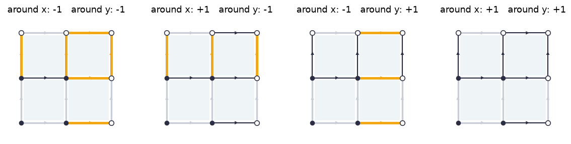
Recap. Averages only see invariants (Fact 3.2). A model is therefore, in effect, a probability distribution on classes, and the probability of a class is proportional to . Some invariants (like the loop products around a torus) are invisible to the faces.
Check yourself
- How many labelings are in each class here? Explain the number.
Answer
There are 8 in each class. There are reframings, but for an abelian group the two constant reframings ( and ) change nothing. So each class has members, and classes.
- As , what does the distribution on classes become?
Answer
It becomes uniform on the four defect-free classes, each with probability . The model has no preference between the loops that go around the board.
- Is the number of defects a quantity the model can "see"? Is the label of edge 3?
Answer
The number of defects is an invariant, so its average is informative. The label of edge 3 is not: it averages to at every .
4. Loop observables on a grid: they decay with area
Recall from Chapter 1 (glossary 3.7) the loop observable of a closed walk : , where is a class function and . It is an invariant, so the model has something to say about it. For the coin model, , so is real.
Here is the question. On a big planar grid, take to be the boundary of an rectangle, walked counterclockwise. How does depend on the rectangle's shape?
Fact 3.3 (a loop is the product of the faces inside). On a planar grid with an abelian label group, the loop product around a rectangle equals the product of the face products of the faces inside it.
Why. Multiply the face products of all the faces inside. Every interior edge is walked once in each direction, by the two faces on either side of it, so its label cancels. Only the boundary is left.
We check this on a random labeling of a grid of vertices (5 × 5 faces):
B6 = Board.grid(6, 6)
face_at = {c: i for i, (c, mu, nu) in enumerate(B6.meta["face_anchor"])}

def rect_walk(a, b, L=6):
    """Vertices around the a-by-b rectangle with corner at the origin, counterclockwise."""
    pts = ([(i, 0) for i in range(a)] + [(a, j) for j in range(b)]
           + [(a - i, b) for i in range(a)] + [(0, b - j) for j in range(b + 1)])
    return [x + L * y for x, y in pts]

U = random_labeling(G, B6, rng)
fp = face_products(G, B6, U)
for a, b in [(1, 1), (1, 2), (2, 3), (3, 4), (4, 4), (5, 5)]:
    inside = [face_at[(x, y)] for x in range(a) for y in range(b)]
    print(f"{a}x{b}:  loop product {int(walk_product(G, B6, U, rect_walk(a, b))):+d}"
          f"   product of faces inside {int(np.prod(fp[inside])):+d}")
1x1: loop product +1 product of faces inside +1
1x2: loop product -1 product of faces inside -1
2x3: loop product +1 product of faces inside +1
3x4: loop product -1 product of faces inside -1
4x4: loop product +1 product of faces inside +1
5x5: loop product +1 product of faces inside +1
Combine Fact 3.3 with Chapter 2's fact that, on a planar grid, the face products are independent, each with average . The average of a product of independent variables is the product of their averages, so:
The prediction is that the average depends on the area only, not on the perimeter .
To test it without leaning on the formula, we measure loop products on samples of the model. A grid has 60 edges, far too many labelings to enumerate. But Chapter 2's independence fact gives an exact sampler:
- Draw every face product independently: with probability .
- Build a labeling with those face products, in tree normal form for a comb-shaped spanning tree (all vertical edges plus the bottom row). Each remaining edge sits directly on top of exactly one face, so its label is fixed by that face's product and the edge below it.
- Apply a uniformly random reframing. Within its class, the model is uniform.
def sample_coin_planar(board, beta, n, rng, reframe_after=True):
    """Exact samples of the coin model on a planar grid. Returns (labelings, face products)."""
    Lx, Ly = board.meta["dims"]; eidx = board.meta["edge_index"]
    fidx = {c: i for i, (c, mu, nu) in enumerate(board.meta["face_anchor"])}
    faces = np.where(rng.random((n, board.n_faces)) < 1 / (1 + np.exp(-2 * beta)), 1, -1).astype(np.int8)
    U = np.ones((n, board.n_edges), dtype=np.int8)         # comb tree edges stay +1
    for y in range(Ly - 1):
        for x in range(Lx - 1):
            below, above = eidx[(x + Lx * y, 0)], eidx[(x + Lx * (y + 1), 0)]
            U[:, above] = faces[:, fidx[(x, y)]] * U[:, below]
    if reframe_after:
        U = reframe(Z2(), board, U, Z2().uniform(rng, (n, board.n_vertices)))
    return U, faces

comb = [e for (v, mu), e in B6.meta["edge_index"].items() if mu == 1 or v < 6]
U_comb, faces = sample_coin_planar(B6, 1.0, 1, rng, reframe_after=False)
print("face products came out as drawn:", np.array_equal(face_products(G, B6, U_comb), faces))
face products came out as drawn: True
Here is one sample before step 3. The grey comb is the spanning tree, where every label is . Read each column of horizontal edges from the bottom up. An edge's label differs from the edge below it exactly when the face between them is a defect (coral).
fig, ax = plt.subplots(figsize=(5.2, 5.2))
viz.draw_board(ax, B6, U_comb[0], G, tree_edges=comb, show_arrows=False,
               title="comb tree normal form (β = 1)")
plt.show()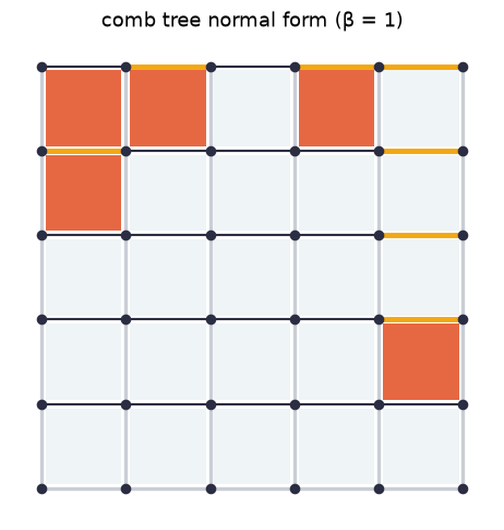
Now we measure. We draw 100,000 exact samples at and average the loop product around every rectangle with . Then we plot two ways: against the area and against the perimeter.
beta = 1.5
Us, _ = sample_coin_planar(B6, beta, 100_000, rng)
shapes, W_avg, W_err = [], [], []
for a in range(1, 6):
    for b in range(a, 6):
        W = walk_product(G, B6, Us, rect_walk(a, b)).astype(float)
        shapes.append((a, b)); W_avg.append(W.mean()); W_err.append(W.std() / np.sqrt(len(W)))
shapes, W_avg, W_err = np.array(shapes), np.array(W_avg), np.array(W_err)
area, perim = shapes.prod(axis=1), 2 * shapes.sum(axis=1)
print("largest deviation from (tanh beta)^area, in standard errors:",
      round(np.max(np.abs(W_avg - np.tanh(beta) ** area) / W_err), 2))
largest deviation from (tanh beta)^area, in standard errors: 2.26
fig, (a0, a1) = plt.subplots(1, 2, figsize=(11.5, 4.3), sharey=True)
logW, logerr = np.log(W_avg), W_err / W_avg
for ax, x, name in [(a0, area, "area  $ab$"), (a1, perim, "perimeter  $2(a+b)$")]:
    ax.errorbar(x, logW, yerr=logerr, fmt="o", color=viz.TEAL, ms=6, capsize=2)
    ax.set_xlabel(name)
xs = np.linspace(0, 26, 50)
a0.plot(xs, xs * np.log(np.tanh(beta)), "--", color=viz.INK, lw=1, label="area · log tanh β")
a0.legend(frameon=False); a0.set_ylabel(r"$\log\langle W_{a\times b}\rangle_\beta$")
for (a, b), x, y in zip(shapes, perim, logW):
    if 2 * (a + b) == 12:
        a1.annotate(f"{a}×{b}", (x, y), xytext=(8, 0), textcoords="offset points", color=viz.CORAL)
a0.set_title("against area: one straight line"); a1.set_title("against perimeter: no single curve")
plt.show()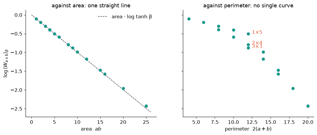
What to look at:
- Left: all 15 shapes fall on a single line through the origin, with slope .
- Right: the three rectangles with perimeter 12 (, , ) have very different averages. The perimeter doesn't determine the answer; the area does.
This clean area behaviour is special to planar boards, where faces are independent. On boards that fill out three or four dimensions it changes, especially at high stiffness. That contrast becomes a central theme in later chapters.
Recap. On a planar grid with an abelian label group, a rectangle's loop product is the product of the faces inside it. Faces are independent, so for the coin model: it decays with area, not perimeter.
Check yourself
- Predict and compare it with the measurement.
Answer
. In the left plot, the point at area sits on the line, at .
- For circle labels with face cost , suppose a single face has . What is for an rectangle on a planar grid?
Answer
The loop angle is the sum of the face angles, which are independent on a planar grid (by the same argument as for coins in Chapter 2). The face angle's distribution is symmetric under , so . Then , so . Again the answer depends on the area only. (Here , a ratio of modified Bessel functions. You won't need this name.)
- Where did the proof of Fact 3.3 use that is abelian?
Answer
The proof cancels each interior edge's label against its inverse. When is non-abelian, the two occurrences aren't next to each other in the product. Face products must first be carried to a common starting vertex (which conjugates them), and only then multiplied together.
5. Non-abelian labels: what the class function sees
For a non-abelian group, a reframing changes a loop product to a conjugate, (Chapter 1). A class function can't tell conjugates apart, so is an invariant.
Take , the permutations of three things, with , the number of points that leaves fixed. This is the trace of 's permutation matrix.
- The identity has .
- The three swaps have .
- The two 3-cycles have .
The board is a grid: one face and four edges. Below, the same labeling is put through five random reframings:
S, B1 = S3(), Board.grid(2, 2)
U = random_labeling(S, B1, rng)
for k in range(5):
    x = face_products(S, B1, reframe(S, B1, U, random_reframing(S, B1, rng)))[0]
    print(f"face product {viz.perm_cycle_notation(S.perm(x)):>6}    chi = {S.chi(x):.0f}")
face product (13) chi = 1
face product (13) chi = 1
face product (23) chi = 1
face product (23) chi = 1
face product (12) chi = 1
The face product jumps around inside one conjugacy class, while stays put.
Now we look at averages. The standard face cost for is . The board has labelings, so we can enumerate them.
- Prediction: the face product is uniform at , and in general is reweighted by .
- So the probability that the face product lands in a conjugacy class is proportional to , where is the value of on .
chi_of = S.chi(S.elements())
kinds = {"identity (χ=3)": 3.0, "swaps (χ=1)": 1.0, "3-cycles (χ=0)": 0.0}
betas = np.linspace(0, 3, 13)
fig, ax = plt.subplots(figsize=(7.5, 4))
for (name, c), col in zip(kinds.items(), [viz.TEAL, viz.GOLD, viz.CORAL]):
    exact = [Model(B1, S, b).exact().average(lambda U: S.chi(face_products(S, B1, U)[:, 0]) == c)
             for b in betas]
    size = np.sum(chi_of == c)
    pred = [size * np.exp(b * c) / sum(np.exp(b * chi_of)) for b in betas]
    ax.plot(betas, pred, color=col, lw=2, label=name)
    ax.plot(betas, exact, "o", color=col, ms=5)
ax.set_xlabel("stiffness β"); ax.set_ylabel("P(face product in conjugacy class)")
ax.legend(frameon=False); ax.set_title("dots: enumeration of 1296 labelings;  lines: prediction")
plt.show()
for b in [0.0, 1.0, 3.0]:
    print(f"beta = {b}:  <chi(U_f)> = {Model(B1, S, b).exact().average(lambda U: S.chi(face_products(S, B1, U)[:, 0])):.3f}")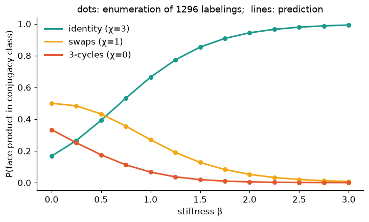
beta = 0.0:  <chi(U_f)> = 1.000
beta = 1.0:  <chi(U_f)> = 2.262
beta = 3.0:  <chi(U_f)> = 2.985
What to look at: as the stiffness grows, the 3-cycles (the most expensive conjugacy class) die out first, then the swaps. The model only ever speaks about the conjugacy class the face product lands in, never about the particular permutation.
Recap. With non-abelian labels, loop products move inside their conjugacy class under reframing. Loop observables are what the model can answer about.
Check yourself
- Why is ?
Answer
At the face product is uniform on . The average number of fixed points is .
- Is for a single edge an invariant? What is its average?
Answer
It is not an invariant: can change the conjugacy class. By Fact 3.1, is uniform, so at every . An average that doesn't move with is a hint (not a proof) that the quantity isn't an invariant.
6. Loop observables pin down the class
Section 3 showed that a model is a distribution on classes. Sections 4 and 5 measured loop observables. Are loop observables enough to tell any two classes apart?
Fact 3.4 (loop observables determine the class). Two labelings of a connected board are in the same class exactly when all of their loop observables agree.
- For an abelian group where labels are numbers (, , circle angles), the loop products themselves serve as the observables.
- For matrix groups, take to be the trace itself, not just its real part. For , the number of fixed points works; we check this on an example below.
Why (abelian case). The loop products of the fundamental cycles are exactly the labels that remain in tree normal form (Chapter 1), and the tree normal form identifies the class. The non-abelian case is harder, so we verify it by brute force instead.
The board for this check is a grid of vertices: 6 vertices, 7 edges and 2 faces. With labels it has labelings. We compute the class of every labeling, and the loop observables of a handful of closed walks at vertex 0. Let be the left face and the right face, both walked from vertex 0. Words like mean "walk , then "; a capital letter means "walk it backwards".
B2 = Board.grid(3, 2)
Us = all_labelings(S, B2)
ids = class_ids(S, B2, Us)
e01 = B2.meta["edge_index"][(0, 0)]                          # the step from vertex 0 to vertex 1
loops = {"a": B2.faces[0], "b": [(e01, 1)] + B2.faces[1] + [(e01, -1)]}
loops["A"], loops["B"] = B2.reverse_walk(loops["a"]), B2.reverse_walk(loops["b"])
words = ["a", "b", "ab", "aB", "abAB"]
FP = np.stack([S.chi(walk_product(S, B2, Us, sum((loops[c] for c in w), []))) for w in words], axis=1)
reps = np.unique(ids, return_index=True)[1]
print(len(Us), "labelings in", len(reps), "classes")
print("fingerprint constant on each class:", np.array_equal(FP, FP[reps][ids]))
print("distinct fingerprints, faces a,b only:", len(np.unique(FP[reps][:, :2], axis=0)))
print("distinct fingerprints, all 5 loops:   ", len(np.unique(FP[reps], axis=0)))
279936 labelings in 11 classes
fingerprint constant on each class: True
distinct fingerprints, faces a,b only: 9
distinct fingerprints, all 5 loops: 11
Here are the 11 classes as rows, each with its fingerprint: the vector in of the values of around the five loops.
- Using only the two faces (left of the bar), some rows coincide: 9 patterns for 11 classes. The rows that coincide are labelled in coral.
- Adding the combined loop makes every row different.
The faces alone don't determine the class. You also need loops that go around several faces, because in a non-abelian group, " then " carries information that and separately don't.
rows = FP[reps]
rows = rows[np.lexsort(rows.T[::-1])]
fig, ax = plt.subplots(figsize=(6.5, 5))
ax.imshow(np.searchsorted([0, 1, 3], rows), cmap=mpl.colors.ListedColormap([viz.PALE, viz.GOLD, viz.TEAL]),
          aspect="auto")
for (i, j), v in np.ndenumerate(rows):
    ax.text(j, i, f"{v:.0f}", ha="center", va="center", color=viz.INK)
ax.axvline(1.5, color=viz.INK, lw=2.5)
ax.set_xticks(range(len(words)), [f"χ({w})" for w in words]); ax.set_yticks(range(len(rows)), [f"class {i+1}" for i in range(len(rows))])
shared = [sum((r[:2] == q[:2]).all() for q in rows) > 1 for r in rows]   # faces alone can't separate
for lab, s in zip(ax.get_yticklabels(), shared):
    lab.set_color(viz.CORAL if s else viz.INK)
ax.set_title("loop fingerprints: faces only | with combined loops"); ax.tick_params(length=0)
for s in ax.spines.values():
    s.set_visible(False)
plt.show()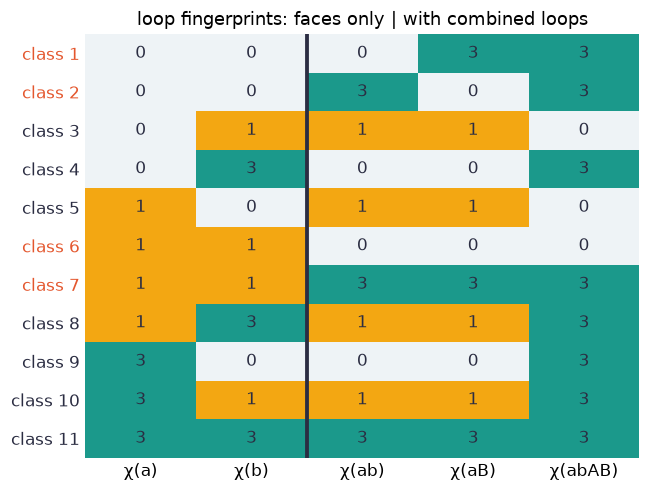
Recap. Loop observables are a complete set of questions. If you know the joint distribution of all of them, you know the model's distribution on classes, and that is everything the model knows.
Check yourself
- For circle labels, take . Do the values over all loops determine the class?
Answer
No. Flip the sign of every angle, so that . Then every loop angle flips too, but its cosine doesn't change. The labelings and are usually in different classes. The fix is to use both and , which amounts to the complex number . That is the full trace of the matrix .
- On the torus from Section 3, which loops do you need besides the faces?
Answer
You need the two loops that go around the board: once horizontally and once vertically. The four calm classes differ only there.
7. Correlations between invariants
Definition (correlation, glossary 4.7). The correlation of two quantities is
If and are independent, the correlation is . Suppose correlations between quantities at distance shrink like for large . Then the number is called the correlation length: it is how far apart two parts of the board must be before they stop "talking".
On a planar grid there is nothing to measure. Below are the exact correlations between the four face products of the grid, at :
def face_corr(board, beta):
    ex = Model(board, G, beta).exact()
    Fp = face_products(G, board, ex.U).astype(float)
    mean = ex.p @ Fp
    return (Fp * ex.p[:, None]).T @ Fp - np.outer(mean, mean)

print("planar 3x3 grid (4 faces):\n", np.round(face_corr(Board.grid(3, 3), 1.0), 6) + 0.0)
print("\n3x3 torus (9 faces), first row:\n", np.round(face_corr(Board.grid(3, 3, periodic=True), 1.0)[0], 6))
planar 3x3 grid (4 faces):
[[0.419974 0. 0. 0. ]
[0. 0.419974 0. 0. ]
[0. 0. 0.419974 0. ]
[0. 0. 0. 0.419974]]
3x3 torus (9 faces), first row:
 [0.351401 0.022217 0.022217 0.022217 0.022217 0.022217 0.022217 0.022217
 0.022217]
What to look at:
- Planar grid: the off-diagonal correlations are exactly , because the faces are independent. The diagonal is the variance .
- Torus: there is a small correlation, the same for every pair of faces, whether they are neighbours or not. It comes from a single global constraint: the product of all face products is . Nothing passes from face to face.
So the boards we have seen have no interesting correlation length. Later chapters use boards that are stacked in layers, or that fill three or four dimensions. There, invariants in different places do influence each other, correlations decay with distance, and the correlation length becomes one of the most important numbers in the course.
Recap. . On planar grids, distinct faces are uncorrelated. On a small torus there is a uniform, distance-free correlation from one global constraint.
Check yourself
- Why is the product of all face products on the torus?
Answer
Every edge lies on exactly two faces, which walk it in opposite directions. So each label appears twice in the product of all face products, as and , and .
- What is on the planar grid?
Answer
It is . At that is , which matches the diagonal.
Chapter recap
- A question to a model is a quantity . The answer is the average .
- Fact 3.1: a single edge label is uniformly distributed at every stiffness. High stiffness calms faces, but never "decides" edges.
- Fact 3.2: averages only see invariants. A model is, in effect, a distribution on classes, with probability proportional to .
- Fact 3.3: on planar grids with abelian labels, a rectangle's loop product is the product of the faces inside it. So for the coin model.
- With non-abelian labels, class functions such as the trace turn loop products into invariants.
- Fact 3.4: loop observables determine the class. Faces alone are not enough: you also need loops that go around several faces, or around the board.
- Correlations between faces vanish on planar grids. Correlation length is a story for layered and higher-dimensional boards.
Dictionary
| Our term | Other names |
|---|---|
| quantity | random variable; observable (physicists reserve this for invariants) |
| average | expectation value; vacuum expectation value (physics) |
| invariant | gauge-invariant observable |
| loop observable | Wilson loop |
| Fact 3.1 (single-edge labels are uniform) | Elitzur's theorem: "a local gauge symmetry cannot be spontaneously broken" |
| reframing average | projection onto the gauge-invariant part |
| area law, Wilson's criterion for confinement (later chapters) | |
| perimeter law | |
| Fact 3.4 (loop observables determine the class) | Giles' theorem (1981) |
| correlation, correlation length | connected correlation function; inverse mass gap (later chapters) |
What's next
This chapter got its numbers in three ways:
- exact enumeration;
- a special exact sampler that only works on planar grids;
- a black-box "sampler" for circle labels.
Chapter 4 opens the black box: sampling by Markov chain Monte Carlo. You build a Markov chain on labelings that makes small local changes and whose long-run distribution is the model (the Metropolis algorithm). You check it against exact enumeration, and you learn how long to wait before its samples are trustworthy.