← Eyal Merhavi · Labelings, models, and gauge theory
Chapter 4 of Labelings, models, and gauge theory, rendered from the executed notebook. Code cells and their outputs are shown as they ran.
Run this chapter in your browser ↗ · Source on GitHub ↗
Runs on JupyterLite. The first time, it downloads Python and its libraries (about 40 MB).
Chapter 4 — Sampling: averages without enumeration
Chapter 3 computed every average by brute force: list every labeling, weigh it, add up. That worked because our boards were tiny. The coin model on a torus has labelings. On a torus it has , about four billion. On a four-dimensional grid with 8 vertices per side it has , a number with almost five thousand digits.
Yet a single average such as "how calm is a typical face?" is just one number. Pollsters estimate what millions of people think by asking a thousand of them. This chapter does the same for models: we learn to draw random labelings from a model and average over the draws. At the end, the method finds something we did not put in: in four dimensions, the coin model makes a sudden jump at a very particular stiffness.
What you'll learn
- Why averages over random samples work, and how to put an error bar on them.
- How to build a Markov chain whose long-run behavior is exactly a given model, using only local information.
- How to tell when a chain has run long enough, and how fast array code makes it.
Prerequisites: chapters 2 and 3 (models, averages, invariants). From probability, we use Markov chains and their stationary distributions.
import time
import numpy as np
import matplotlib.pyplot as plt

from lgt import *
from lgt import viz
from lgt.grid import GridModel

viz.use_style()
rng = np.random.default_rng(4)
Helpers for this chapter. mean_face is
the invariant we will estimate throughout: the average over faces of
.
For the coin model it equals
,
so 1 means "all calm" and 0 means "half the faces are defects".
def mean_face(G, board, U):
    """Average over faces of chi(face product). Works on a batch of labelings."""
    return G.chi(face_products(G, board, U)).mean(axis=-1)

def running_mean(x):
    return np.cumsum(x) / np.arange(1, len(x) + 1)
4.1 Averages from samples
Fix a model and an invariant . Suppose we could draw labelings independently from . The sample average
is a random number. The law of large numbers says , and the central limit theorem says how fast: the typical error is , where is the variance of under the model. The error does not depend on how many labelings exist. Four billion or , a thousand samples give about three correct digits.
Let's watch it happen where we still know the exact answer: the coin model on the torus ( labelings), at . We draw independent samples straight from the exact distribution (cheating, for now) and track the running average.
T3 = Board.grid(3, 3, periodic=True)
M3 = Model(T3, Z2(), beta=0.5)
ex = M3.exact()
f_all = mean_face(Z2(), T3, ex.U)                       # f for every labeling
exact = float(np.sum(ex.p * f_all))
sigma = float(np.sqrt(np.sum(ex.p * (f_all - exact) ** 2)))
draws = f_all[rng.choice(len(ex.p), size=4000, p=ex.p)]  # 4000 independent samples
print(f"exact <mean face> = {exact:.4f},  sigma = {sigma:.3f}")
print(f"sample average of 4000 draws = {draws.mean():.4f}")
exact <mean face> = 0.4638, sigma = 0.299
sample average of 4000 draws = 0.4597
n = np.arange(1, len(draws) + 1)
fig, ax = plt.subplots(figsize=(7, 3.6))
ax.fill_between(n, exact - 2 * sigma / np.sqrt(n), exact + 2 * sigma / np.sqrt(n),
                color=viz.TEAL, alpha=0.18, label=r"exact $\pm 2\sigma/\sqrt{n}$")
ax.plot(n, running_mean(draws), color=viz.INK, lw=1.4, label="running sample average")
ax.axhline(exact, color=viz.CORAL, lw=1.5, ls="--", label="exact average")
ax.set(xscale="log", xlabel="number of samples $n$", ylabel="mean face", ylim=(exact - 0.3, exact + 0.3))
ax.legend(loc="upper right", fontsize=9)
plt.show()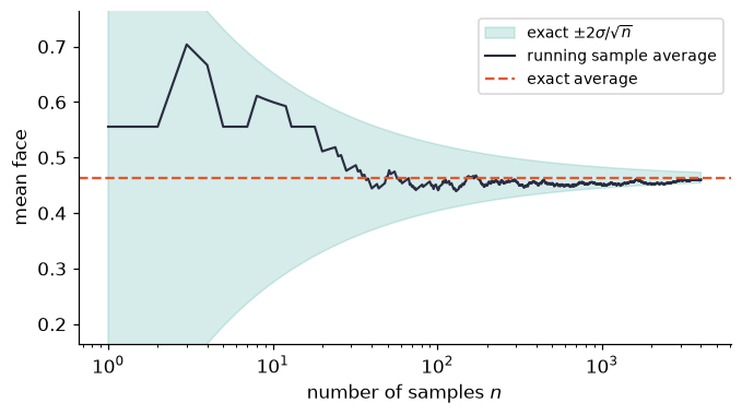
The black curve wanders early and then stays inside the shaded funnel, which narrows like . That funnel is the whole promise of sampling.
Recap. If we can draw independent samples from , the sample average of an invariant converges to with error about , no matter how many labelings there are.
Check yourself
- How many samples do you need to cut the error by a factor of 10?
Answer
100 times as many, because the error shrinks like .
- We just drew samples using
ex.p, the list of all probabilities. Why can't we do that on the torus?
Answer
Computing those probabilities needs the normalizer , a sum over all labelings, and storing them needs one number per labeling. The next section avoids both.
4.2 A random walk that settles into the model
We cannot draw independent samples without knowing . But we can compare two labelings: the ratio
needs no , only the difference in total cost. The idea of Markov chain Monte Carlo is to take a random walk on the set of labelings , moving from to with probabilities chosen so that, in the long run, the walk spends a fraction of its time at each .
Fact 4.1 (detailed balance). If for all pairs of labelings, then is a stationary distribution of the chain. If moreover the chain can reach every labeling from every other one, and is not periodic, then the distribution of the walk after steps converges to from any starting point.
Why the first part: sum both sides over . The left side is the probability of being at after one step when starting from ; the right side is . The second part is the convergence theorem for finite Markov chains.
The Metropolis rule. One step of the walk:
- pick an edge (for example, in random order);
- propose a new label for , drawn uniformly from ;
- compute the change in total cost ;
- accept the proposal with probability ; otherwise keep the old label.
Moves that lower the cost are always accepted, and moves that raise it are accepted sometimes. You can check detailed balance in one line: for , .
The crucial practical point is that step 3 is cheap.
Fact 4.2 (locality). Changing the label of one edge changes only the face products of the faces that use . So is a sum over those faces alone: 2 faces on a square grid, on a -dimensional grid, no matter how big the board is.
P4 = Board.grid(4, 4)
e = P4.meta["edge_index"][(5, 0)]                      # an interior horizontal edge
touch = [1.0 if e in [e2 for e2, _ in f] else 0.0 for f in P4.faces]
fig, ax = plt.subplots(figsize=(4, 4))
viz.draw_board(ax, P4, face_values=touch, face_cmap="Greys", highlight_walk=[(e, 1)],
               title="one edge, and the only faces it touches")
ax.collections[0].set_alpha(0.35)
plt.show()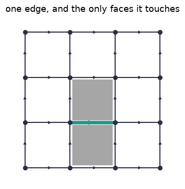
The teal edge appears in exactly two faces (shaded). To decide whether to change its label, the walk looks at nothing else.
Let's test the whole recipe against exact enumeration. The library's
Model.metropolis implements it. On the
torus the exact distribution of the total cost is known, so we
compare.
T2 = Board.grid(2, 2, periodic=True)
M2 = Model(T2, Z2(), beta=0.5)
ex2 = M2.exact()
chain = M2.metropolis(rng, n_samples=6000, burn_in=200)
for S in np.unique(ex2.cost):
    exact_p = ex2.p[ex2.cost == S].sum()
    chain_p = np.mean(np.isclose(M2.cost(chain), S))
    print(f"total cost {S:>4.0f}: exact {exact_p:.3f}   Metropolis {chain_p:.3f}")
total cost 0: exact 0.546 Metropolis 0.547
total cost 4: exact 0.444 Metropolis 0.442
total cost 8: exact 0.010 Metropolis 0.011
The frequencies agree to about two decimals, which is what 6000 (correlated) samples can deliver.
Recap. A Markov chain that satisfies detailed balance with respect to and can reach every labeling eventually samples from . The Metropolis rule achieves this using only cost differences, so is never needed, and each step only looks at the faces through one edge.
Check yourself
- At , what does the Metropolis chain do?
Answer
Every proposal is accepted (), so each visited edge gets a fresh uniform label. After one sweep the labeling is uniform, matching the model at .
- On a 4-dimensional grid, how many faces must be examined to update one edge?
Answer
. Each of the 3 other directions gives one face "on each side" of the edge.
- Does the chain care that the model is unchanged by reframings?
Answer
No. It wanders through labelings, including many in the same class, and that is harmless: the class probabilities come out right because the labeling probabilities do. Invariant averages are all we read off.
4.3 Face remainders and the heat bath
For one edge , walk any face through it starting with in its stored direction. The face product splits as
where the face remainder is the product of the face's other labels (glossary 4.8). With everything except held fixed, the cost of the edge is , a function of alone.
For the coin model this is especially simple. With , the part of the total cost that involves is , where
is the sum of the remainders. So instead of proposing and maybe rejecting, we can draw the new label directly from its exact conditional distribution:
This is the heat bath update (statisticians call it Gibbs sampling). The conditional probability is a logistic curve in : the faces around the edge "vote", and sets how much the edge listens.
fig, ax = plt.subplots(figsize=(6, 3.4))
A = np.linspace(-2.2, 2.2, 200)
for beta, c in zip([0.25, 0.5, 1.0], [viz.MUTED, viz.TEAL, viz.CORAL]):
    ax.plot(A, 1 / (1 + np.exp(-2 * beta * A)), color=c, label=fr"$\beta={beta}$")
    ax.plot([-2, 0, 2], 1 / (1 + np.exp(-2 * beta * np.array([-2, 0, 2]))), "o", color=c)
ax.set(xlabel="sum of face remainders $A(e)$ (2D: one of $-2,0,2$)",
       ylabel=r"$\Pr(U(e)=+1)$")
ax.legend()
plt.show()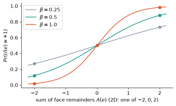
On a square grid can only be , or (the dots). When both faces "want" , a stiff model obeys almost surely; when they disagree (), the edge flips a fair coin at every stiffness.
A heat-bath sweep on a board takes a few lines. For the coin model inverses are trivial, so a remainder is just the product of the other labels on the face.
def heat_bath_sweep(board, U, beta, rng, faces_of=None):
    faces_of = faces_of or board.faces_of_edge()
    for e in rng.permutation(board.n_edges):
        A = sum(np.prod([U[e2] for e2, _ in board.faces[f] if e2 != e]) for f in faces_of[e])
        U[e] = 1 if rng.random() < 1 / (1 + np.exp(-2 * beta * A)) else -1
    return U

U = random_labeling(Z2(), T2, rng)
vals = [mean_face(Z2(), T2, heat_bath_sweep(T2, U, 0.5, rng)) for _ in range(4000)]
print(f"heat bath: {np.mean(vals[200:]):.4f}   exact: {ex2.average(lambda X: mean_face(Z2(), T2, X)):.4f}")
heat bath: 0.5318 exact: 0.5363
Recap. The face remainder is "the rest of the face" seen from edge . The cost of one edge depends only on the remainders of its faces. For the coin model the conditional distribution of a label is logistic in their sum, and the heat bath samples from it directly.
Check yourself
- On a 3D grid, which values can take?
Answer
Each edge lies on faces, each remainder is , so .
- Does a heat-bath update ever "reject"?
Answer
No. It always draws a new label, but the new label may well equal the old one. Its long-run behavior is the same model; it is often a little more efficient than Metropolis.
4.4 Many edges at once
The Python loop above visits edges one by one. Fact 4.2 suggests something better: two edges that share no face can be updated at the same time, because neither one's update depends on the other's label. On a grid we can split the edges into groups of this kind:
- edges pointing in the same direction never share a face if they are not neighbors "sideways";
- so group the direction- edges by the parity (even/odd) of the sum of their other coordinates.
That gives groups, each updated in one shot with array arithmetic. (On a torus this needs even side lengths, so the parity pattern wraps around consistently.)
B6 = Board.grid(6, 6)
cols = {(0, 0): viz.TEAL, (0, 1): viz.GOLD, (1, 0): viz.CORAL, (1, 1): viz.INK}
fig, ax = plt.subplots(figsize=(4.6, 4.6))
viz.draw_board(ax, B6, faces=False, show_arrows=False, edge_labels=None)
for (v, mu), e2 in B6.meta["edge_index"].items():
    par = sum(B6.meta["coord"][v][nu] for nu in range(2) if nu != mu) % 2
    (x0, y0), (x1, y1) = B6.pos[B6.edges[e2]]
    ax.plot([x0, x1], [y0, y1], color=cols[(mu, par)], lw=4, solid_capstyle="round", zorder=5)
ax.set_title("4 update groups: same colour = no shared face")
plt.show()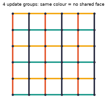
Check any face: its four edges have four different colors. So all teal edges can be redrawn at once, then all gold, and so on.
The library's GridModel (in lgt.grid)
stores a labeling of a
-dimensional
torus as an array and runs exactly this scheme: heat bath for the coin
model, Metropolis for the circle. First, it gives the right answer:
G2 = GridModel((2, 2), Z2(), beta=0.5).hot_start(rng)
G2.sweep(rng, 200)
fast = [(G2.sweep(rng), G2.mean_face())[1] for _ in range(8000)]
print(f"GridModel: {np.mean(fast):.4f}   exact: {ex2.average(lambda X: mean_face(Z2(), T2, X)):.4f}")
GridModel: 0.5384 exact: 0.5363
Second, it is fast. Here is the time per sweep (every edge updated once) on an torus:
T8 = Board.grid(8, 8, periodic=True)
t = time.perf_counter(); Model(T8, Z2(), 0.5).metropolis(rng, 5, burn_in=0); slow = (time.perf_counter() - t) / 5
G8 = GridModel((8, 8), Z2(), 0.5).hot_start(rng)
t = time.perf_counter(); G8.sweep(rng, 200); quick = (time.perf_counter() - t) / 200
print(f"edge-by-edge Python: {1e3 * slow:.1f} ms/sweep   arrays: {1e3 * quick:.2f} ms/sweep   "
      f"speed-up ~{slow / quick:.0f}x")
edge-by-edge Python: 2.8 ms/sweep arrays: 0.10 ms/sweep speed-up ~27x
Recap. Edges that share no face can be updated simultaneously. On a -dimensional torus with even sides, parity groups suffice, which turns a sweep into a handful of array operations.
GridModeldoes this and agrees with exact enumeration.
Check yourself
- Why can't a horizontal and a vertical edge be in the same group in general?
Answer
They can lie on a common face (every face has two horizontal and two vertical edges), and then updating one changes the remainder seen by the other.
- On a torus the parity trick breaks. Why?
Answer
Going around an odd cycle of length 3 returns you to the start after an odd number of parity flips, so some pair of neighbors gets the same parity and shares a face.
4.5 How long is long enough?
A Markov chain has two weaknesses that independent samples do not have.
It starts somewhere. Early samples remember the starting labeling. We throw away a burn-in period. A good test: start two chains far apart, one from the identity labeling (every face calm, "cold") and one from a uniform random labeling ("hot"), and watch them meet. Below: the coin model on an torus at two stiffnesses.
fig, ax = plt.subplots(figsize=(7, 3.4))
for beta, ls in [(0.6, "-"), (0.74, "--")]:
    for start, c in [("cold", viz.TEAL), ("hot", viz.CORAL)]:
        M = GridModel((8, 8, 8), Z2(), beta)
        M.cold_start() if start == "cold" else M.hot_start(rng)
        trace = [(M.sweep(rng), M.mean_face())[1] for _ in range(150)]
        ax.plot(trace, color=c, ls=ls, lw=1.4, label=f"{start} start, β={beta}")
ax.set(xlabel="sweeps", ylabel="mean face")
ax.legend(fontsize=8, ncol=2)
plt.show()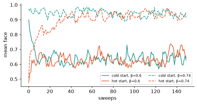
At the two chains meet within a few sweeps. At they take much longer: the model is near a point where it changes character (section 4.6), and the chain moves sluggishly there.
It remembers. Consecutive samples are correlated, so chain samples are worth fewer than independent ones. The autocorrelation of the series at lag is , and the integrated autocorrelation time measures how many sweeps one effective sample costs: correlated samples carry about as much information as independent ones.
def autocorr(x, kmax):
    x = np.asarray(x) - np.mean(x)
    return np.array([np.mean(x[: len(x) - k] * x[k:]) for k in range(kmax)]) / np.var(x)

def tau_int(rho):
    s = 0.5
    for k in range(1, len(rho)):
        if rho[k] < 0.05: break
        s += rho[k]
    return s
fig, ax = plt.subplots(figsize=(6.5, 3.4))
series = {}
for beta, c in [(0.6, viz.TEAL), (0.70, viz.CORAL)]:
M = GridModel((8, 8, 8), Z2(), beta).hot_start(rng); M.sweep(rng, 300)
series[beta] = np.array([(M.sweep(rng), M.mean_face())[1] for _ in range(8000)])
rho = autocorr(series[beta], 80)
ax.plot(rho, color=c, lw=2, label=fr"$\beta={beta}$: $\tau\approx{tau_int(rho):.1f}$ sweeps")
ax.axhline(0, color=viz.MUTED, lw=0.8)
ax.set(xlabel="lag $k$ (sweeps)", ylabel=r"$\rho(k)$")
ax.legend()
plt.show()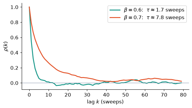
Closer to the special stiffness the memory is longer: about four times longer at than at . It keeps growing as you approach . At even 16,000 sweeps are not enough for the estimates below to settle. This slowdown is a real obstacle in practice, and whole families of cleverer algorithms exist to fight it.
Error bars that respect memory: binning. Chop the series into blocks of length and average each block. Once the block averages are nearly independent, and the ordinary formula is honest. Plotting that estimate against , it grows and then levels off at the true error.
def binned_error(x, b):
    m = len(x) // b
    blocks = np.asarray(x[: m * b]).reshape(m, b).mean(axis=1)
    return blocks.std(ddof=1) / np.sqrt(m)

bs = 2 ** np.arange(0, 10)
fig, ax = plt.subplots(figsize=(6.5, 3.4))
for beta, c in [(0.6, viz.TEAL), (0.70, viz.CORAL)]:
    ax.plot(bs, [binned_error(series[beta], b) for b in bs], "o-", color=c, label=fr"$\beta={beta}$")
ax.set(xscale="log", yscale="log", xlabel="block length $b$", ylabel="estimated error of the mean")
ax.legend()
plt.show()
for beta in series:
    print(f"beta={beta}: mean face = {series[beta].mean():.4f} ± {binned_error(series[beta], 256):.4f}")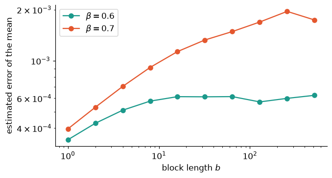
beta=0.6: mean face = 0.6277 ± 0.0006
beta=0.7: mean face = 0.7900 ± 0.0020
Reading the plateau gives an honest error bar. The naive estimate () understates the error, and the closer you are to the special stiffness, the worse it gets. If the curve never levels off, the honest conclusion is that the run is too short.
Recap. Discard a burn-in (start hot and cold; wait until they agree). Consecutive samples are correlated; the integrated autocorrelation time says how many sweeps one effective sample costs. Binning gives error bars that account for the correlation.
Check yourself
- A run of 10,000 sweeps has . About how many independent samples is it worth?
Answer
.
- Why does the binned error estimate grow with before it levels off?
Answer
For small , neighboring blocks are still correlated, so their spread underestimates how much the overall mean can wander. As passes the blocks decorrelate and the estimate reaches the true error.
4.6 A first experiment, and a puzzle
We now have a tool that works on boards far too large to enumerate. Let's use it to ask a simple question in three settings: how does the mean face change as we turn the stiffness dial? We use the coin model on tori of dimension 2, 3 and 4.
To look for surprises we sweep slowly up, carrying the chain's labeling from one to the next, and then slowly back down. If the model behaves smoothly, the two passes agree.
def scan(dims, betas, equil, measure, rng):
    M = GridModel(dims, Z2(), betas[0]).hot_start(rng)
    out = {}
    for name, bs in [("up", betas), ("down", betas[::-1])]:
        vals = []
        for b in bs:
            M.beta = b
            M.sweep(rng, equil)
            vals.append(np.mean([(M.sweep(rng), M.mean_face())[1] for _ in range(measure)]))
        out[name] = np.array(vals if name == "up" else vals[::-1])
    return out
runs = {2: ((32, 32), np.linspace(0.1, 1.2, 12)),
3: ((12, 12, 12), np.linspace(0.55, 0.95, 9)),
4: ((8, 8, 8, 8), np.linspace(0.38, 0.50, 13))}
results = {d: scan(dims, bs, equil=150, measure=40, rng=rng) for d, (dims, bs) in runs.items()}fig, axs = plt.subplots(1, 3, figsize=(14, 3.9))
for ax, (d, (dims, bs)) in zip(axs, runs.items()):
ax.plot(bs, results[d]["up"], "o-", color=viz.TEAL, label=r"$\beta$ going up")
ax.plot(bs, results[d]["down"], "s--", color=viz.CORAL, mfc="none", label=r"$\beta$ going down")
ax.set(title=f"{d} dimensions, " + "×".join(map(str, dims)), xlabel=r"stiffness $\beta$")
axs[0].plot(runs[2][1], np.tanh(runs[2][1]), color=viz.INK, lw=1, label=r"$\tanh\beta$ (chapter 2)")
axs[0].set_ylabel("mean face")
axs[2].axvline(0.5 * np.log(1 + np.sqrt(2)), color=viz.INK, ls=":", lw=1.2)
axs[2].text(0.5 * np.log(1 + np.sqrt(2)) + 0.002, 0.6, " ?", fontsize=14)
for ax in axs: ax.legend(fontsize=8, loc="lower right")
plt.show()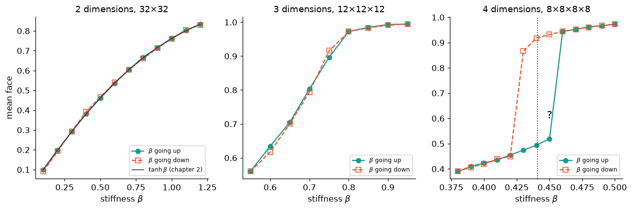
Three very different pictures.
- 2 dimensions: a smooth curve, exactly , as chapter 2 predicted (faces are nearly independent on a large torus).
- 3 dimensions: a smooth but steep rise near . Up and down agree.
- 4 dimensions: the two passes disagree. Going up, the model stays "rough" until about , then jumps; going down, it stays "calm" until about , then falls. In between, where the model ends up depends on where it came from. This memory effect is called hysteresis, and it is the fingerprint of an abrupt change: two very different typical behaviors, each stable enough that a local chain cannot cross from one to the other.
The puzzle. The dotted line is at , right where the two branches separate. Where would such a number come from? Nothing in our definitions mentions . Chapter 9 shows that it can be derived, without any simulation: a short exact argument (a Fourier transform on ) shows that the 4D coin model at stiffness is secretly the same as the 4D coin model at another stiffness , with . The only stiffness that is its own partner is , and that is where the jump must be. The 3D steep rise has a similar exact explanation, with a different partner model.
Recap. The array sampler lets us study big tori. Turning the stiffness up and down reveals that dimension matters: smooth in 2D, steep in 3D, and an abrupt, hysteretic jump in 4D, located at a number we will derive exactly.
Check yourself
- Why do we carry the labeling from one to the next instead of restarting each time?
Answer
To make memory visible. Restarting would hide which branch the chain was on. (For accurate averages away from the jump, either way works once burn-in is done.)
- Would a longer run make the 4D loop disappear?
Answer
It shrinks slowly, but on a large board crossing between the two behaviors requires the whole board to reorganize, which a local chain essentially never does. The 3D curve, in contrast, already agrees in both directions.
- Check the self-partner claim: solve .
Answer
Write . Then , so , i.e. and . So .
Chapter recap
- Averages of invariants can be estimated from random samples, with error independent of the number of labelings.
- A Markov chain obeying detailed balance samples a model without ever computing . Metropolis proposes and accepts with ; the heat bath draws from the exact conditional distribution.
- Locality: one edge's update needs only its face remainders, of them on a -dimensional grid. Edges sharing no face can be updated together, which makes array code fast.
- Chains need a burn-in and have memory: the autocorrelation time sets the cost of an effective sample, and binning gives honest error bars.
- In 4D the coin model shows hysteresis at a stiffness near , a number chapter 9 derives exactly.
Dictionary
| Our term | Other names |
|---|---|
| Markov chain Monte Carlo | MCMC; "Monte Carlo simulation" (physics) |
| Metropolis rule | Metropolis(–Hastings) algorithm |
| heat bath | Gibbs sampling (statistics) |
| face remainder , sum | staple, sum of staples (physics) |
| sweep | one update of every edge; a "lattice sweep" |
| burn-in | thermalization, equilibration |
| cold / hot start | ordered / disordered start |
| slow memory near a special | critical slowing down |
| hysteresis, abrupt jump | first-order phase transition |
| partner stiffness | Kramers–Wannier / Wegner duality; self-dual point |
History: the 4D jump was found exactly this way, by Creutz, Jacobs and Rebbi (1979), in one of the first computer studies of these models.
What's next
So far a model has been a static object: a distribution over whole labelings. Chapter 5 starts Part II, where we cut a board into layers and ask how one layer constrains the next. On the simplest boards, chains of vertices, a model is a Markov chain in disguise, and one matrix, the transfer matrix, holds all of its secrets.