← Eyal Merhavi · Labelings, models, and gauge theory
Chapter 6 of Labelings, models, and gauge theory, rendered from the executed notebook. Code cells and their outputs are shown as they ran.
Run this chapter in your browser ↗ · Source on GitHub ↗
Runs on JupyterLite. The first time, it downloads Python and its libraries (about 40 MB).
Chapter 6 — Yang–Mills and the Millennium problem, in our terms
In 2000 the Clay Mathematics Institute listed seven problems, each with a million-dollar prize. One of them is about physics: prove that quantum Yang–Mills theory exists and has a mass gap. It is usually stated in the language of quantum field theory: operator-valued distributions, Hilbert spaces, the Wightman axioms. That language takes years to learn.
This chapter shows that you already have almost everything you need to state the problem precisely. Yang–Mills theory on a grid is one of our models: a particular label group, a particular board, the standard face cost. The Millennium problem asks what happens to that model as the grid is refined. We will see where the physicists' formulas come from, run the experiment that first convinced physicists the picture is right, and end with a precise statement of what was proved in 2026 and what is still open.
What you'll learn
- Why physics uses the groups , , , and that lattice Yang–Mills is our model with on a four-dimensional grid.
- Why the standard face cost is the right one, and how it becomes the physicists' "curvature" for smooth labelings, including the term that exists only because the labels don't commute.
- Why four dimensions is special, and how a length scale appears out of nowhere (asymptotic freedom).
- The Millennium problem, stated in the vocabulary of chapters 0–5, and its status as of November 2026.
- What this elementary framework is missing for non-commutative physics: Lie algebras, representations, and how charges combine into invariants.
Prerequisites: chapters 0–5. We use the layering and the levels of chapter 5 only in the last sections.
import numpy as np
import matplotlib.pyplot as plt
from scipy.special import iv

from lgt import *
from lgt import viz
from lgt.grid import GridModel

viz.use_style()
rng = np.random.default_rng(6)
G = SU2()
6.1 The label group of nature
The groups in physics' Standard Model are , which we have met as the circle, and the matrix groups
is the label group of the strong force, which holds atomic nuclei together. We will work with the smallest case, , because it already has everything that matters: it is compact, so it has a uniform distribution (chapter 2), and it is non-abelian, so reframing genuinely changes loop products, by conjugation (chapter 1).
has a friendly concrete form. Every element is for a unit vector , where are three fixed matrices (the Pauli matrices). So is the 3-sphere , the matrix product, written in these coordinates, is the multiplication rule of the quaternions, and the trace is . The library stores labels exactly this way.
a, b = G.uniform(rng, 2)
M = G.to_matrix
print("a b as matrices equals the matrix of the quaternion product:",
      np.allclose(M(G.mul(a, b)), M(a) @ M(b)))
print("ab = ba ?", np.allclose(G.mul(a, b), G.mul(b, a)), "   tr(a) = 2w:", np.isclose(G.chi(a), 2 * a[0]))
a b as matrices equals the matrix of the quaternion product: True
ab = ba ? False tr(a) = 2w: True
Why these groups? The physics, at a high level
The interlude after chapter 1 gave the recipe. If some property of a particle can only be described relative to a convention, and every point of space may choose its convention independently, then comparing neighbors forces labels on edges. The label group is the group of convention changes for that property. So "which label group?" means "which hidden property, and how can its conventions be changed?" Physics answers this by experiment, three times:
| Force | Hidden property, and its conventions | Label group |
|---|---|---|
| electromagnetism | the phase of a charged particle's wavefunction: a unit complex number, with no preferred zero angle | , the circle |
| weak force | a two-valued "which partner?" label: the electron and its neutrino (and the up and down quarks, the constituents of protons and neutrons) behave as two components of one vector in | |
| strong force | color: every quark carries a vector in , with no preferred basis ("red, green, blue" is a convention) |
A little history shows where non-commuting labels came from. In 1932 Heisenberg, noting that the proton and the neutron have almost the same mass, proposed treating them as two states of one particle. By 1937 experiments showed that they also feel the nuclear force almost identically, and this became a symmetry: the pair is one vector in , and the force is unchanged when it is rotated by (physicists call this isospin). In 1954 Yang and Mills asked our interlude's question about it: what if every point could choose its own convention for which component is the proton? The answer was labels in a non-commuting group. That is where the name of this chapter comes from. Their own application did not survive: isospin is only an approximate symmetry, and their theory predicted massless force carriers that nobody had seen. But the structure later described both the weak and the strong force.
Why three colors? Nobody sees color directly, so the evidence is indirect, and it all says 3:
- a particle called the is, in the simplest quark picture, three up quarks in the same state. Quarks are fermions, particles that quantum mechanics forbids from sharing a state with an identical twin (the Pauli exclusion principle). The puzzle disappears if the three quarks differ in a hidden label with at least three values;
- when an electron and a positron (its antiparticle) collide, they sometimes produce hadrons (particles made of quarks) and sometimes a pair of muons (heavier cousins of the electron). The ratio of the two rates is three times what it would be without color, up to small corrections;
- the neutral pion (a light particle made of quarks) decays into two photons, the particles of light, at a rate proportional to the square of the number of colors, and the measured rate matches 3.
And no free colored particle has ever been seen: only color-neutral combinations. In our language, only invariants are observed. That is chapter 3's statement that a model knows only averages of invariants, now as an experimental fact (physicists call it confinement of color).
Why "S" and "U"?
- U (unitary, ): a change of color convention must preserve the length of the color vector, because the length carries probability. Unitary matrices are exactly the length-preserving ones.
- S (determinant 1): the remaining freedom in , an overall phase , changes all three colors alike, so it is not a change of color convention at all. Including it would add a ninth force carrier that pulls on every quark equally, and no such force is seen; phases are left to the separate circle factor. Determinant 1 also has a structural consequence, which we will compute in section 6.6: three quarks can combine into an invariant. Protons and neutrons are built this way.
- Not real rotations (): quarks and antiquarks (their antiparticles) carry genuinely different kinds of color charge, which needs complex vectors. With real rotations they would transform identically, and two quarks could already combine into an invariant (their dot product). Such two-quark particles are not seen.
To be honest about the limits of this story: these arguments explain what kind of group fits each force, and they simplify. The weak acts on only one "handedness" of each particle and is hidden at everyday energies, and the Standard Model's circle factor is not exactly electromagnetism's but mixes with . Nor do the arguments explain why nature chose rather than something else. That remains an experimental input.
Definition (lattice Yang–Mills). The lattice Yang–Mills model with group is the model of chapter 2 with
- board: a four-dimensional torus grid, faces the unit squares;
- label group: ;
- face cost: the standard one, ;
- stiffness: .
That is the whole definition. Everything in chapters 1–5 applies: classes, invariants, loop observables, sampling, layers and levels. Physicists write the same model with the cost and stiffness , so . For , . We quote both when comparing with the literature.
Recap. is the 3-sphere of unit quaternions; it is compact and non-abelian. Lattice Yang–Mills is our model on a 4D torus with and the standard face cost.
Check yourself
- What is the face cost of an element in terms of its quaternion ?
Answer
. It is 0 exactly at the identity and largest, 4, at .
- Why can't a model be built with , all invertible real matrices?
Answer
is not compact (matrices can be arbitrarily large), so it has no uniform probability distribution to build on, for the same reason as the exchange rates of chapter 0.
- Why does the label group of color need complex matrices, rather than real rotations of ?
Answer
Quarks and antiquarks carry different kinds of color. In a reframing acts on an antiquark by the complex conjugate of the matrix that acts on a quark, and for that is genuinely different. With real rotations the two would transform identically, and two quarks could form an invariant, which is not seen.
- Color is never observed directly. How does that fit the framework of chapter 3?
Answer
Color is a convention at each point, so a color vector by itself is not an invariant. A model only knows averages of invariants, and experiments only ever see color-neutral combinations: the same statement, read physically.
6.2 From faces to curvature
Physicists do not describe Yang–Mills theory with labels on edges. They use a gauge field : at every point of space, in every direction , a small "infinitesimal rotation" (for ). Our labelings are the discrete version. Put the grid at spacing and set
where
turns a small rotation vector into a group element
(
in quaternions; the library's SU2.exp). The labels are then
all close to the identity, and change slowly from edge to edge.
What does our total cost become for such labels? Here is the answer first. It uses a field built from and its derivatives, the curvature, which Step 2 below constructs.
Fact 6.1 (faces become curvature). For slowly varying labels on a -dimensional grid of spacing , the total cost is .
We derive it in three steps.
Step 1: the cost of a label close to the identity
For , has quaternion and trace . So the standard cost of a label near the identity is
The cost of a face whose product is is just the squared length of the rotation vector .
Step 2: the face product of slowly varying labels
Walk around the face at in the plane of directions . Its product is
Two separate effects make differ from the identity.
(a) The field changes from edge to edge. If the labels commuted, multiplying exponentials would just add their vectors. The sum is , and a first-order Taylor expansion turns it into
This is the "circulation around a small square" from vector calculus, the curl.
(b) The labels don't commute. Even if the field is constant, with and everywhere, the face product is . For numbers this would be exactly 1. For rotations it is not. Let's measure it.
def qlog(q):
    """Inverse of SU2.exp: the rotation vector v in R^3 with exp(v) = q."""
    w, v = np.clip(q[..., 0], -1, 1), q[..., 1:]
    n = np.linalg.norm(v, axis=-1, keepdims=True)
    return np.arccos(w)[..., None] * v / np.where(n > 0, n, 1)

a_vec, b_vec = np.array([0.3, -0.5, 0.8]), np.array([0.6, 0.2, -0.4])
print("2 a x b =", np.round(2 * np.cross(a_vec, b_vec), 4))
for eps in [0.2, 0.1, 0.05, 0.025]:
    ea, eb = G.exp(eps * a_vec), G.exp(eps * b_vec)
    face = G.mul(G.mul(G.mul(ea, eb), G.inv(ea)), G.inv(eb))        # around one face, constant field
    print(f"eps = {eps:<6} rotation vector of the face product / eps^2 = {np.round(qlog(face) / eps ** 2, 4)}")
2 a x b = [0.08 1.2 0.72]
eps = 0.2 rotation vector of the face product / eps^2 = [-0.0585 1.044 0.9121]
eps = 0.1 rotation vector of the face product / eps^2 = [0.0102 1.1295 0.8239]
eps = 0.05 rotation vector of the face product / eps^2 = [0.0451 1.1669 0.7737]
eps = 0.025 rotation vector of the face product / eps^2 = [0.0626 1.184 0.7472]
As shrinks, the face product's rotation vector divided by approaches , with an error that halves along with :
Fact 6.2 (small loops measure non-commutativity). For small rotation vectors, , where for the bracket is .
The space of small rotation vectors, here, together with this bracket is what mathematicians call the Lie algebra of the group. The bracket is the infinitesimal shadow of non-commutativity. It vanishes for the circle, where every two labels commute. (The general tool behind Fact 6.2 is the Baker–Campbell–Hausdorff formula.)
To order the two effects simply add: the bracket in (b) is already of order , so evaluating the field at the face's corner instead of at each edge changes it only at order . So the face product is up to smaller terms, where
The first two terms are effect (a); the cross product is effect (b), and it exists only because the labels don't commute. Physicists call the curvature or field strength.
Step 3: add up the faces
By Step 1, each face costs about . A -dimensional region of unit volume contains about grid vertices, and one face per vertex in each plane . So summing over faces is times integrating:
This is Fact 6.1. The integral is the Yang–Mills energy (physicists: the Yang–Mills action). Let's verify Fact 6.1 in two dimensions, where , using a smooth field of our choosing.
def A_field(x, y):
    """A smooth SU(2) gauge field on the unit square: two R^3-valued functions."""
    a1 = np.stack([np.sin(2 * np.pi * y), 0.5 * np.cos(2 * np.pi * x), 0 * x], -1)
    a2 = np.stack([0 * x, np.sin(2 * np.pi * x) * np.cos(2 * np.pi * y), 0.7 + 0 * x], -1)
    return a1, a2

def curvature(x, y, with_cross=True, h=1e-5):
    a1, a2 = A_field(x, y)
    d1a2 = (A_field(x + h, y)[1] - A_field(x - h, y)[1]) / (2 * h)
    d2a1 = (A_field(x, y + h)[0] - A_field(x, y - h)[0]) / (2 * h)
    return d1a2 - d2a1 + (2 * np.cross(a1, a2) if with_cross else 0)
def smooth_labeling(n):
"""The labeling U(x -> x + eps e_mu) = exp(eps A_mu(x)) on an n x n torus, eps = 1/n."""
B = Board.grid(n, n, periodic=True)
U = np.empty((B.n_edges, 4))
for (v, mu), e in B.meta["edge_index"].items():
x, y = np.array(B.meta["coord"][v]) / n
U[e] = G.exp(A_field(np.array(x), np.array(y))[mu] / n)
return B, U
xs = (np.arange(1000) + 0.5) / 1000
X, Y = np.meshgrid(xs, xs, indexing="ij")
YM = np.mean(np.sum(curvature(X, Y) ** 2, -1))
YM_no_cross = np.mean(np.sum(curvature(X, Y, with_cross=False) ** 2, -1))
print(f"Yang-Mills energy: {YM:.3f} (if labels commuted, it would be {YM_no_cross:.3f})")Yang-Mills energy: 31.084 (if labels commuted, it would be 29.609)
ns = [8, 16, 32, 64, 128]
ratios = []
for n in ns:
    B, U = smooth_labeling(n)
    S = np.sum(2 - G.chi(face_products(G, B, U)))
    ratios.append(S * n ** 2 / YM)                       # S / eps^2, relative to the integral
    print(f"grid {n:>3}x{n:<3}  total cost / eps^2 = {S * n**2:8.4f}   ratio to integral = {ratios[-1]:.4f}")
grid 8x8 total cost / eps^2 = 29.0928 ratio to integral = 0.9359
grid 16x16 total cost / eps^2 = 30.5790 ratio to integral = 0.9838
grid 32x32 total cost / eps^2 = 30.9572 ratio to integral = 0.9959
grid 64x64 total cost / eps^2 = 31.0521 ratio to integral = 0.9990
grid 128x128 total cost / eps^2 = 31.0759 ratio to integral = 0.9997
B, U = smooth_labeling(16)
fc = 2 - G.chi(face_products(G, B, U))
anch = [np.array(a[0]) / 16 + 0.5 / 16 for a in B.meta["face_anchor"]]
Fc = np.array([np.sum(curvature(np.array(p[0]), np.array(p[1])) ** 2) for p in anch]) / 16 ** 4
fig, axs = plt.subplots(1, 3, figsize=(14, 4.2), layout="constrained")
norm = plt.Normalize(0, max(fc.max(), Fc.max()))
viz.draw_board(axs[0], B, face_values=fc, face_cmap="magma_r", face_norm=norm, show_arrows=False,
               vertex_size=4, title="face costs of the labeling (16×16)")
viz.draw_board(axs[1], B, face_values=Fc, face_cmap="magma_r", face_norm=norm, show_arrows=False,
               vertex_size=4, title=r"$\varepsilon^4|F_{12}|^2$ at each face centre")
axs[2].loglog([1 / n for n in ns], np.abs(1 - np.array(ratios)), "o-", color=viz.TEAL)
axs[2].loglog([1 / n for n in ns], 4 * np.array([1 / n for n in ns]) ** 2, "--", color=viz.MUTED, label=r"slope 2: error $\propto\varepsilon^2$")
axs[2].set(xlabel=r"grid spacing $\varepsilon$", ylabel="relative error of Fact 6.1", title="convergence")
axs[2].legend()
plt.show()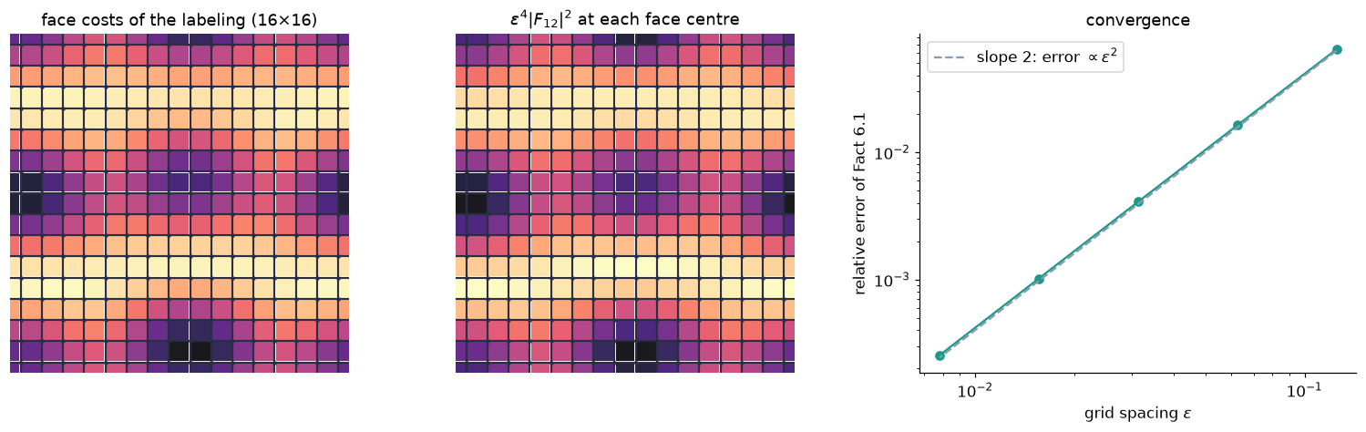
The left two panels are the same picture: the cost of each face is the local curvature, face by face. On the right, the relative error falls by a factor of 4 each time the grid is refined by 2, so it shrinks like . And the limit is the integral with the cross term: the non-commutativity of the labels is not a detail, it is visible in the total cost.
The rest of the physicists' dictionary follows the same pattern:
| Our term | Continuum Yang–Mills |
|---|---|
| labeling , labels | gauge field (connection) |
| reframing , with | gauge transformation |
| face product | curvature, field strength |
| total cost | Yang–Mills action (times ) |
| loop observable | Wilson loop |
| model | the Euclidean path integral |
Why this face cost?
The standard face cost can look arbitrary. It isn't. Here are the requirements it meets, each one forced by something earlier in the course:
- Reframing-invariant. A model must not depend on conventions (chapter 2). The cost has to be an invariant, and the most local building blocks are face products. (Locality is what makes sampling cheap in chapter 4 and gives the transfer matrix of chapter 5; costs that couple distant faces lose both.)
- A class function. Reframing changes a face product by conjugation, (chapter 1). So must satisfy . For this means depends only on the rotation angle of the face product, not on its axis. The trace is the simplest class function there is.
- Smallest at the identity, and only there. Calm faces should be preferred, so consistent labelings are the most likely.
- The right behavior near the identity. Step 1 of section 6.2 used . That is what makes the total cost become the Yang–Mills energy.
- Flip-positive. Its weight expands in characters with nonnegative coefficients (chapter 5, section 5.6), so the derived system exists.
Requirement 4 hides the deepest point: only the bottom of the bowl matters. For smooth labelings, every face product is near the identity, and there any cost meeting requirements 2–4 looks like . Far from the identity, different costs disagree, but the continuum limit is believed not to care. The picture below compares candidates for the circle group, where a face product is an angle .
th = np.linspace(-np.pi, np.pi, 400)
n_hk = np.arange(-20, 21)
heat = np.exp(-n_hk ** 2 / 2) @ np.cos(np.outer(n_hk, th))           # heat kernel on the circle at time 1
costs = {r"standard: $1-\cos\theta$": 1 - np.cos(th),
         r"quadratic: $\theta^2/2$": th ** 2 / 2,
         r"heat kernel: $-\log K(\theta)/K(0)$": -np.log(heat / heat.max()),
         r"bad: $\frac{1}{4}(1-\cos 2\theta)$": (1 - np.cos(2 * th)) / 4}
fig, ax = plt.subplots(figsize=(8, 4))
ax.axvspan(-0.5, 0.5, color=viz.PALE, zorder=0)
for (lab, c), col in zip(costs.items(), [viz.INK, viz.TEAL, viz.GOLD, viz.CORAL]):
    ax.plot(th, c, color=col, lw=2.5 if "quadratic" in lab else 2,
            ls="--" if "bad" in lab else ":" if "quadratic" in lab else "-", label=lab, zorder=3 if "quadratic" in lab else 2)
ax.text(0, 2.6, "smooth labelings\nlive here", ha="center", fontsize=9, color=viz.MUTED)
ax.set(xlabel=r"face product angle $\theta$", ylabel=r"cost $\varphi$", ylim=(0, 3.2))
ax.legend(fontsize=9, loc="upper right")
plt.show()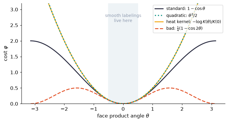
In the shaded region near the first three costs are indistinguishable: all are . (The quadratic and heat-kernel costs stay close over the whole range shown; the standard cost bends away beyond about .) They differ far from the identity, where smooth labelings never go. The dashed coral cost also matches near 0, but it fails requirement 3: it has a second minimum at , so it would also reward faces whose product is , and it describes a different theory.
Physicists have a name for "only the bottom of the bowl matters": universality. All costs that agree near the identity, and meet the other requirements, are believed to give the same continuum limit; they differ only in how fast the grid approaches it. Each variant has its uses:
- the heat-kernel cost makes the 2D model exactly unchanged when a face is subdivided, so in 2D every grid already gives the continuum answer;
- improved costs add small rectangles with tuned weights, which cancels the leading error of Fact 6.1, so coarser grids already look continuous;
- the standard cost, introduced by Kenneth Wilson in 1974, is the simplest, and it is what we have used.
Why is itself the right continuum energy? Run the same requirements on continuum expressions. The energy must be built from (and its derivatives), because itself carries the conventions. It must be unchanged by reframings, local, and unchanged by rotations of space. Among such expressions, is the simplest one. In 4D it is also the only one whose stiffness is a pure number (section 6.3); every more complicated expression, such as , gets suppressed by extra powers of as the grid is refined. (There is one exception: a "topological" term, called the -term, whose value does not change under small changes of the field. It is outside this course.)
Recap. For slowly varying labels , a face costs about when its product is , and face products become , so the total cost becomes , the Yang–Mills energy (verified, error ). The cross term in is the bracket of Fact 6.2: it exists because the labels don't commute. The standard cost is the simplest one meeting the requirements (invariant, class function, minimum only at the identity, nearby, flip-positive); by universality, other such costs give the same continuum limit.
Check yourself
- For the circle group , what is ?
Answer
, with no cross term, because angles commute. This is the electromagnetic field: Yang–Mills is Maxwell's theory of light.
- Fact 6.1 is about smooth labelings. Are typical samples from the model smooth?
Answer
No. Typical samples are rough at every scale (chapter 4's pictures at moderate are full of defects). Fact 6.1 explains why the cost function is the right one, not what typical samples look like. That gap is exactly where the difficulty of the Millennium problem lives.
6.3 Why four dimensions is special
Look at the power of in Fact 6.1. The model's weight is
To describe a fixed continuous picture as the grid is refined, the combination should stay fixed. In or that means grows as in a definite way. But in the spacing cancels: is a pure number, and nothing in the formula says how big anything is. Classically, four-dimensional Yang–Mills has no built-in length scale. A theory with no length scale cannot have a mass gap: there is no length to set the size of a lightest particle.
Yet the model on the grid does have a length: its correlation length , measured in grid steps (chapter 5's inverse gap). The resolution is that the naive scaling is wrong. The randomness of the labels at short distances changes how must be tuned. The physicists' computation, done by hand in 1973 by Gross, Wilczek and Politzer, says that to keep the physics fixed while refining, the stiffness must grow, slowly:
Here is a length scale that the theory creates: it is not in the definition. This is asymptotic freedom: as the grid gets finer the stiffness goes to infinity, so on short scales the labels are nearly consistent. The number comes from counting how the non-commuting labels interact, which is the cross term in (Fact 6.2) at work. Equivalently, the area-law rate per face (the rate in chapter 3's decay ; physicists call it the "string tension" in grid units) should fall like .
What "running" means, concretely
The phrase "the stiffness must grow" is easy to say and hard to picture. Here it is step by step.
- Pick something physical to hold fixed. For example, the correlation length: how far apart two faces must be before their behaviors become (nearly) independent. Measure it in physical units, say .
- On the grid, the model measures it in grid steps. The model at stiffness has some correlation length in grid steps, the inverse of chapter 5's gap. In physical units that is .
- Refine the grid without changing the physics. Keeping while forces . The model must be tuned to stiffer and stiffer values, where its correlations reach across more and more grid steps.
- How fast? Asymptotic freedom says grows exponentially with , like . So refining by a factor 2 costs only an additive , and grows like : logarithmically slowly.
Why must grow, rather than shrink? Here is a heuristic picture, not a proof; the direction of the effect is the output of the 1973 calculation, not something you can see without it. Imagine viewing a fine grid from twice as far away, by combining the labels of each block of faces into "coarse" labels. For non-commuting groups the random wiggles of the fine labels interact with each other, through the cross term of Fact 6.2, and their net effect is to make the coarse labels rougher than the fine ones: the coarse grid behaves like a model with a smaller stiffness. So to make the coarse picture match a given target, the fine grid must start stiffer. Physicists call this anti-screening, and counting the contributions is the calculation that produced the 11.
The direction depends on the group. For the circle alone, the wiggles at different scales do not interact (at large in 4D the model is nearly Gaussian) and the stiffness does not run at all. In real electromagnetism, pairs of charged particles make it run the other way: the effective stiffness grows at long distances, and electric charge looks weaker from far away (physicists call this screening).
The experimental signature: at very short distances, which means at very high energies, quarks inside a proton behave as if they were almost free. This was seen in electron–proton collisions at the Stanford Linear Accelerator Center (SLAC) from 1968 onward ("deep inelastic scattering", Nobel Prize 1990 for Friedman, Kendall and Taylor), before the theory explained it. Gross, Wilczek and Politzer received the 2004 Nobel Prize for the explanation.
Recap. In 4D the total cost of a smooth labeling does not depend on the spacing, so classically there is no length scale. Asymptotic freedom says the stiffness must grow logarithmically as the grid is refined, and a length scale appears from the randomness itself.
Check yourself
- Halving the grid spacing at fixed physics: by how much must grow (leading order, )?
Answer
From : . Every halving costs the same small additive step, so only logarithmically.
- In 2D, how must scale with to keep fixed?
Answer
fixed, so : it grows like the number of faces per unit area.
6.4 What the computer says
In 1979–80 Michael Creutz ran exactly the experiment of chapter 4 on 4D , with a machine slower than your phone. Two findings convinced physicists that lattice Yang–Mills is the right object.
Finding 1: no jump. Recall the 4D coin model: sweeping up and down gave a hysteresis loop, an abrupt change between two behaviors. If had such a jump, the region of small (where the area law is proven, see below) would be cut off from the region of large (where the continuum lives), and lattice results would say nothing about the continuum. Let's look.
def scan(dims, G_, betas, equil, measure, rng):
    M = GridModel(dims, G_, betas[0]).hot_start(rng)
    out = {}
    for name, bs in [("up", betas), ("down", betas[::-1])]:
        vals = []
        for b in bs:
            M.beta = b
            M.sweep(rng, equil)
            vals.append(np.mean([(M.sweep(rng), M.mean_face())[1] for _ in range(measure)]))
        out[name] = np.array(vals if name == "up" else vals[::-1])
    return out

b_su2 = np.linspace(0.5, 1.6, 12)
su2 = scan((6, 6, 6, 6), G, b_su2, equil=40, measure=15, rng=rng)
b_z2 = np.linspace(0.38, 0.50, 13)
z2 = scan((6, 6, 6, 6), Z2(), b_z2, equil=60, measure=20, rng=rng)
fig, axs = plt.subplots(1, 2, figsize=(11, 3.8))
for ax, bs, res, title in [(axs[0], b_z2, z2, r"4D coin model ($\mathbb{Z}_2$)"),
(axs[1], b_su2, su2, r"4D $SU(2)$ (lattice Yang–Mills)")]:
ax.plot(bs, res["up"], "o-", color=viz.TEAL, label=r"$\beta$ going up")
ax.plot(bs, res["down"], "s--", color=viz.CORAL, mfc="none", label=r"$\beta$ going down")
ax.set(title=title, xlabel=r"stiffness $\beta$", ylabel="mean face")
ax.legend(loc="lower right", fontsize=9)
plt.show()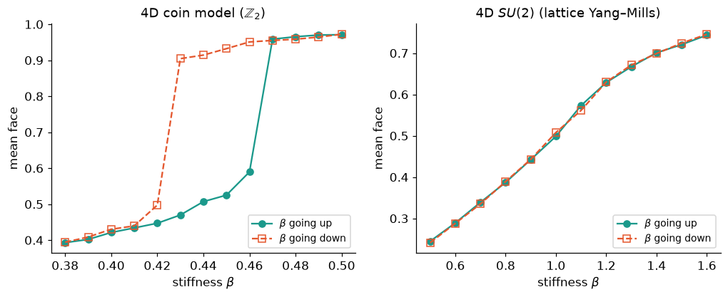
Left: the jump of chapter 4. Right: rises smoothly, and the two passes lie on top of each other. (Sanity check against the literature: at , physicists' , the published mean face is .)
Finding 2: from strong coupling (physicists' name for small ) to asymptotic freedom. Measure the area-law rate. A clean way to extract it from small loops is the Creutz ratio
where is the average loop observable of an rectangle. If (a perimeter part and an area part), the perimeter parts cancel in the ratio and . We know two limits:
- small : faces are nearly independent, as in 2D (chapter 3), so with (a ratio of Bessel functions, exact for one face), giving ;
- large : asymptotic freedom predicts , with one unknown constant (the scale of section 6.3).
def creutz_22(beta, rng, dims=(6, 6, 6, 6), equil=60, measure=80):
    M = GridModel(dims, G, beta).hot_start(rng)
    M.sweep(rng, equil)
    W = {k: [] for k in [(1, 1), (1, 2), (2, 2)]}
    for _ in range(measure):
        M.sweep(rng)
        for k in W:
            W[k].append(M.mean_rectangle(*k))
    w = {k: np.mean(v) for k, v in W.items()}
    return -np.log(w[(2, 2)] * w[(1, 1)] / w[(1, 2)] ** 2)

betas_c = np.array([0.7, 0.8, 0.9, 1.0, 1.1, 1.2, 1.25])
chi = np.array([creutz_22(b, rng) for b in betas_c])
for b, c in zip(betas_c, chi):
    print(f"beta = {b:.2f} (physicists' {2 * b:.2f}):  chi(2,2) = {c:.3f}")
beta = 0.70 (physicists' 1.40): chi(2,2) = 1.102
beta = 0.80 (physicists' 1.60): chi(2,2) = 0.995
beta = 0.90 (physicists' 1.80): chi(2,2) = 0.775
beta = 1.00 (physicists' 2.00): chi(2,2) = 0.618
beta = 1.10 (physicists' 2.20): chi(2,2) = 0.389
beta = 1.20 (physicists' 2.40): chi(2,2) = 0.247
beta = 1.25 (physicists' 2.50): chi(2,2) = 0.201
bb = np.linspace(0.6, 1.4, 200)
strong = -np.log(iv(2, 2 * bb) / iv(1, 2 * bb))
C = chi[-1] / np.exp(-12 * np.pi ** 2 * betas_c[-1] / 11)        # fix the one unknown constant
af = C * np.exp(-12 * np.pi ** 2 * bb / 11)
fig, ax = plt.subplots(figsize=(7, 4.2))
ax.semilogy(bb, strong, color=viz.GOLD, lw=2, label=r"small-$\beta$ prediction $-\ln\,I_2(2\beta)/I_1(2\beta)$")
ax.semilogy(bb, af, color=viz.INK, lw=1.5, ls="--", label=r"asymptotic freedom $\propto e^{-12\pi^2\beta/11}$")
ax.semilogy(betas_c, chi, "o", color=viz.TEAL, ms=8, label=r"measured $\chi(2,2)$, $6^4$ torus")
ax.set(xlabel=r"stiffness $\beta$ (physicists' $\beta$ is $2\beta$)", ylabel="area-law rate per face",
       ylim=(0.05, 3))
ax.legend(fontsize=9)
plt.show()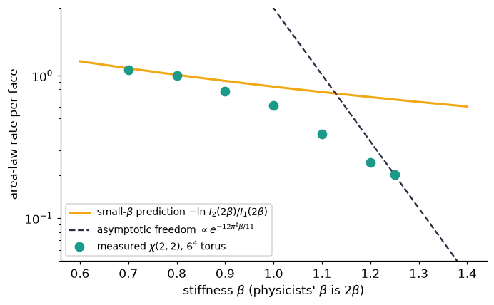
At small the measurements sit on the gold strong-coupling curve. As grows they peel away from it and bend toward the dashed asymptotic-freedom line, crossing over smoothly, with no jump. This is Creutz's 1980 picture, and it was the first evidence that the confining behavior at small (physicists call the area law confinement) and the asymptotically free behavior at large belong to one theory.
Be honest about what the plot does not show. The points have not settled onto the dashed line's slope: at these stiffnesses the loops are only one or two grid steps across, and corrections are large. Physicists know this well; reaching true asymptotic scaling took larger boards, larger and better methods, and is still checked carefully today.
Recap. On a 4D torus, shows no jump between small and large , unlike the coin model. The area-law rate follows the exact small- curve and then crosses over toward the asymptotic-freedom prediction, as Creutz first saw in 1980.
Check yourself
- Why do the perimeter parts cancel in ?
Answer
Perimeters: has , has , together ; has . Areas: versus , leaving exactly one unit of area.
- Why does "no jump" matter for the continuum?
Answer
The continuum is reached at , and the area law is easy to prove at small . A jump in between would mean the provable, confining region tells you nothing about the continuum region. Smoothness suggests (it does not prove) that confinement survives all the way.
6.5 The Millennium problem, in our terms
Here is the plan of the construction, using only words from this course.
The refinement. Fix a compact, simple, non-abelian label group (for example or ). For a spacing , take the four-dimensional torus grid of spacing and side (in physical units), with the standard face cost and some stiffness . This is a model in the sense of chapter 2: an honest probability distribution on , a finite product of copies of (of 3-spheres, for ). Then send and .
Existence. Show that can be chosen so that:
- averages of invariants (suitably smoothed loop observables) converge as , ;
- the limit is nontrivial: not the model where all labels are consistent, and not a "free" (Gaussian) model;
- the limit keeps flip-positivity (chapter 5, glossary 5.7), which survives limits;
- the limit gains the full symmetry of 4D space: all rotations and translations, not only the quarter-turns and whole-step shifts of the grid.
Given 1–4, the construction of chapter 5 (state space from functions of a layer, ) goes through in the limit. Physicists call this Osterwalder–Schrader reconstruction, and the result is what they mean by "quantum Yang–Mills theory on ".
Mass gap. In the limit, the derived system has levels , and the problem asks to show
In grid language: the gap measured in grid units, , times the inverse spacing, stays bounded away from zero, . Equivalently, the correlation length measured in physical units, , stays bounded (it tends to ). Physically: the lightest particle of the theory (a "glueball", a lump of pure field) has a positive mass, even though the classical theory has no length scale at all (section 6.3).
Chatterjee's survey Yang–Mills for probabilists states the probabilistic core as three problems (its Problems 4.1, 5.1 and 5.2), which now read naturally. Each is about any infinite-volume limit of the 4D model, for non-abelian :
| Problem | In our words |
|---|---|
| Area law (4.1) | Rectangle loop observables are bounded by at every (not only small ). |
| Mass gap (grid) (5.1) | For every , correlations of two face observables decay like with , and as . |
| Continuum limit (5.2) | As there are , and a constant with : after removing a perimeter part, rescaled loop observables have a nontrivial limit. |
What is known (status as of November 2026).
| Statement | Status |
|---|---|
| Area law and positive gap at small , any , any dimension | Proved (Osterwalder–Seiler 1978, using expansions in powers of ). |
| 2D: everything, exactly, at every | Proved; the 2D model is a random walk on (chapter 5) and its continuum limit can be computed exactly. |
| 4D existence (items 1–4 above, with infinite volume reached along a subsequence) | Announced by OpenAI (October 2026), formalized in the Lean proof assistant. On November 10, 2026 a review panel chaired by David Gross (with Douglas, Jaffe, Klebanov, Nekrasov) affirmed it; the panel did not claim to fully understand the proof. |
| Uniqueness of the infinite-volume limit | Open. |
| 4D mass gap | Open. |
| 4D area law at large (confinement) | Open. |
Why did existence fall first? Roughly, existence is mostly about short distances, where asymptotic freedom makes the model nearly consistent and expansions around consistency are better behaved. The gap and the area law are about long distances, where the model is genuinely random and no known method has control. The picture below summarizes the landscape along the stiffness axis.
fig, ax = plt.subplots(figsize=(11, 2.6))
ax.axvspan(0, 0.9, color=viz.GOLD, alpha=0.25)
ax.axvspan(0.9, 1.4, color=viz.MUTED, alpha=0.15)
ax.axvspan(1.4, 2.5, color=viz.TEAL, alpha=0.2)
ax.plot(betas_c, 0.24 + 0 * betas_c, "o", color=viz.INK, ms=4)
ax.text(betas_c.mean(), 0.31, "β values simulated above", ha="center", fontsize=8, color=viz.INK)
for x, txt in [(0.45, "small β: rough, confining\narea law + gap PROVED"),
               (1.15, "crossover\n(no jump: measured)"),
               (1.95, "large β: nearly consistent\ncontinuum lives at β → ∞\nexistence: 2026; gap: OPEN")]:
    ax.text(x, 0.5, txt, ha="center", va="center", fontsize=10)
ax.annotate("", xy=(2.5, 0.08), xytext=(0, 0.08), arrowprops=dict(arrowstyle="->", color=viz.INK))
ax.text(2.48, 0.16, "stiffness β", ha="right", fontsize=10)
ax.set(xlim=(0, 2.5), ylim=(0, 1)); ax.axis("off")
plt.show()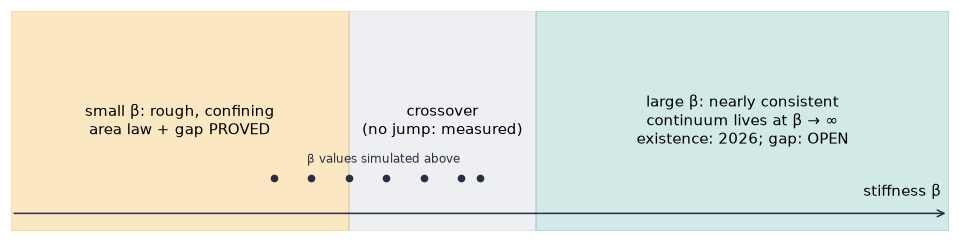
The picture is schematic: the region boundaries are only indicative. The dots are the stiffnesses we simulated. Everything the Millennium problem asks lives at the right edge, and it asks for control uniformly as you move right forever.
Recap. The Millennium problem, in our words: refine a 4D model with a tuned stiffness; show averages of invariants converge to a nontrivial, flip-positive, rotation-symmetric limit (existence), and that the derived system's gap stays positive in physical units (mass gap). Small and 2D are understood; 4D existence was affirmed in November 2026; the gap is open.
Check yourself
- Which property of chapter 5 guarantees that the limit, if it exists, has a positive Hamiltonian?
Answer
Flip-positivity (glossary 5.7). It makes the transfer matrix symmetric with nonnegative eigenvalues, so is defined and bounded below, and it survives limits because it is an inequality between averages.
- Why isn't rotation symmetry automatic?
Answer
The grid only has quarter-turn rotations. Full rotation symmetry has to emerge in the limit, which is part of what must be proved.
- A grid model at fixed has a finite correlation length. Why isn't that already a mass gap?
Answer
The gap must be positive in physical units after refinement. As we need in grid units, at exactly the rate ; a finite at one says nothing about that limit.
6.6 What our elementary framework is missing
Everything in chapters 0–5 works for any compact group, commuting or not: labelings, reframings, classes, models, sampling, layers. So in one sense the framework already handles non-commutative labels. But physics with non-commuting groups uses several tools we never built. Some appeared in this chapter in disguise. Here they are, in roughly the order you would need them.
1. The infinitesimal picture: Lie algebras
Section 6.2 used "small rotation vectors" , the map , and the bracket , all defined by hand for . The general theory is the Lie algebra of a group: the vectors that turns into group elements near the identity, with the bracket from Fact 6.2. It is what lets you write a continuum field , a continuum reframing , and the curvature for any group. For the Lie algebra has dimension : 3 for , and 8 for . Those 8 directions are the 8 kinds of gluon, the particles that carry the strong force as photons carry electromagnetism.
2. Charged fields that are vectors: representations
The interlude's charged field had one complex number per vertex, which is enough for the circle. A quark carries a color vector, , and a reframing acts on it by a matrix. With written as a row vector, the rule that keeps the interlude's formulas unchanged is
The covariant difference has the same formula as before, , with now a matrix. A way for a group to act by matrices on vectors is called a representation. A group has many representations, and different particles live in different ones:
- quarks are in the defining representation ;
- gluons themselves are in the adjoint representation: the Lie algebra, of dimension , on which acts by conjugation, .
The loop observables of chapter 3 can then be taken in any representation: becomes the trace of the loop product as it acts in that representation. Different representations give different area-law rates. In 2D, for , the adjoint rate approaches times the defining one as (and equals it exactly for the heat-kernel cost).
3. Building invariants from several charges
Experiments only see invariants. With vector-valued charges, which combinations are invariants? Two examples show the pattern.
A quark and an antiquark joined by a string. Take a quark at , with color vector , and a walk from to . An antiquark at is described by a column vector , the conjugate transpose of a row vector that reframes like a quark; since is unitary, . The number
is an invariant. The reframings at and cancel against the endpoints of the walk product, the same telescoping as in chapter 1. A single quark has no invariant at all, but a quark–antiquark pair joined by a path of labels does. Physicists call such a pair a meson. The string of labels between them is the precise sense in which charges in a gauge theory are never fully local, and chapter 3's area law is the cost of stretching that string.
Two (or three) quarks at one point. For , two color vectors (rows) at the same vertex give the invariant
because a reframing multiplies the matrix on the right by , which multiplies its determinant by . Here is where the "S" of earns its place: for unitary matrices with , this would not be an invariant. For the same construction with three color vectors gives the invariant : three quarks combine into a color-neutral particle, a baryon. Protons and neutrons are baryons.
M = G.to_matrix
B9 = Board.grid(3, 3)
U9, h9 = random_labeling(G, B9, rng), random_reframing(G, B9, rng)
U9r = reframe(G, B9, U9, h9)
psi9 = rng.normal(size=(9, 2)) + 1j * rng.normal(size=(9, 2))                 # a quark field: C^2 per vertex
psi9r = np.array([psi9[v] @ np.linalg.inv(M(h9[v])) for v in range(9)])       # reframed: psi h^{-1}
walk = B9.walk([0, 1, 2, 5, 8])                                               # from corner 0 to corner 8
string = lambda U, p: p[0] @ M(walk_product(G, B9, U, walk)) @ p[8].conj()
print("quark-string-antiquark:  before", np.round(string(U9, psi9), 5), "  after", np.round(string(U9r, psi9r), 5))
quark-string-antiquark: before (-2.52467+4.60494j) after (-2.52467+4.60494j)
psi, chi = psi9[4], rng.normal(size=2) + 1j * rng.normal(size=2)
h_su2 = M(G.uniform(rng))
h_u2 = np.exp(0.7j) * h_su2                                                   # unitary, but det = e^{1.4 i}
det2 = lambda p, c: np.linalg.det(np.array([p, c]))
for name, hm in [("SU(2) reframing", h_su2), ("U(2) reframing ", h_u2)]:
    hi = np.linalg.inv(hm)
    print(f"{name}: det before {np.round(det2(psi, chi), 4)}   after {np.round(det2(psi @ hi, chi @ hi), 4)}")
SU(2) reframing: det before (0.841+1.5746j) after (0.841+1.5746j)
U(2) reframing : det before (0.841+1.5746j) after (1.6946-0.5611j)
The string invariant survives the reframing exactly. The determinant survives an reframing but not one with .
Classifying all the ways to build invariants from several representations is the subject of representation theory: tensor products, characters, and their orthogonality. It is the main mathematical tool we skipped. It also powers the exact solution of the 2D model for non-commuting groups (a random walk on , diagonalized by characters, just as section 5.7 did for the circle), the expansion behind flip-positivity (section 5.6), and predictions such as the ratio between the area-law rates of adjoint and defining loops in 2D (a ratio of two numbers attached to each representation, and ).
4. Two things that need more than new tools
- Quarks are fermions. Their path-integral variables anticommute (Grassmann variables), so their "weights" are not probabilities. They can be integrated out into a determinant, but that determinant is not always positive (it is in the cases lattice simulations of the strong force mostly use, but not, for example, for matter at high density), which breaks the stance "a model is a probability distribution". Putting them on a grid also hits a no-go theorem (Nielsen–Ninomiya): under natural assumptions, left-right asymmetric matter like the weak force's cannot be put on a grid directly.
- Topology. Smooth fields with labels in , the 3-sphere, can wind around the group in ways no small smooth change can undo (instantons). They carry the -term mentioned in section 6.2 and are invisible to the face-by-face reasoning of this course. (On a grid the winding is only approximately defined, since any labeling can be deformed continuously into any other.)
Recap. To go beyond pure Yang–Mills on a grid you need: Lie algebras (the infinitesimal side: small rotation vectors and the bracket), representations (charged fields that are vectors; quarks in , gluons in the Lie algebra), and representation theory (which combinations of charges are invariant: mesons as quark–string–antiquark, baryons as determinants, which is why matters). Fermions and topology need genuinely new ideas.
Check yourself
- How many gluons does have, and why?
Answer
8, the dimension of its Lie algebra: anti-Hermitian matrices with trace 0 form a real vector space of dimension .
- Why is a single quark not an invariant, while is?
Answer
A reframing multiplies by , which changes it. In the string expression, the from the quark cancels the at the start of the walk product, and the at the end of the walk product cancels the from the antiquark.
- With instead of as the label group, could three quarks form an invariant?
Answer
Not by the determinant: it would pick up the factor , a phase that need not be 1.
Course recap
- Chapter 0: a currency market is a board with labels; round trips are the only meaningful numbers; changing units is a reframing.
- Chapter 1: for any group, labelings modulo reframings are classes; invariants are functions of classes; loop products change by conjugation; the tree normal form removes the redundancy.
- Chapter 2: a model is a probability distribution over labelings, built on the uniform distribution of a compact group; redundancy costs nothing.
- Chapter 3: a model knows only averages of invariants; single labels average to zero; loop observables reveal the area law.
- Chapter 4: Markov chains sample models using only local information, and found a jump at a number we can derive, .
- Chapter 5: cutting a board into layers turns a model into a transfer matrix; its levels, the "quantum system", are derived from the distribution alone.
- Chapter 6: physics' label groups are the convention-change groups of hidden properties (phase, weak partner, color). Yang–Mills is our model with ; the standard cost is the simplest valid one and becomes curvature for smooth labels, with a term that exists only because labels don't commute. 4D has no built-in scale until asymptotic freedom creates one; the Millennium problem is a statement about refining that model. Going further needs Lie algebras and representation theory.
Dictionary
| Our term | Physics |
|---|---|
| board: 4D torus grid of spacing | Euclidean spacetime with a lattice cutoff |
| label group | gauge group (color group; for the strong force) |
| labeling, | gauge field, link variables |
| reframing | gauge transformation |
| face product, | plaquette, field strength / curvature |
| standard face cost | Wilson action |
| "only the bottom of the bowl matters" | universality |
| small rotation vectors with the bracket | Lie algebra, commutator, structure constants |
| color vector at a vertex, | quark field in the fundamental representation |
| quark–string–antiquark invariant | gauge-invariant meson operator |
| determinant of color vectors | baryon (color singlet of quarks) |
| coarse labels rougher than fine ones | anti-screening; running coupling |
| stiffness | ( the coupling); physicists' |
| total cost for smooth labels | Yang–Mills action |
| loop observable | Wilson loop |
| area-law rate | string tension |
| Creutz ratio | Creutz ratio |
| stiffness growing as the grid refines | asymptotic freedom, running coupling |
| length scale created by the model, | , dimensional transmutation |
| refining the grid with tuned | continuum limit, renormalization |
| derived system of the limit | quantum Yang–Mills theory (Osterwalder–Schrader reconstruction) |
| gap in physical units | mass gap; lightest glueball mass |
Where to go next
- Sourav Chatterjee, Yang–Mills for probabilists (arXiv:1803.01950): the closest text to this course's point of view.
- Michael Creutz, Quarks, Gluons and Lattices (1983): the computational story, by the person who first ran it.
- Erhard Seiler, A gentle introduction to lattice field theory (Entropy, 2025), and the classic review by John Kogut (Rev. Mod. Phys., 1979).
- Arthur Jaffe and Edward Witten, Quantum Yang–Mills Theory: the official Clay problem statement.
- The 2026 existence proof:
- the Lean code as submitted, yang-mills-group/OpenAI-YM-20261028;
- the shepherding committee's validation, yang-mills-group/YM, with its assessment;
- this course's reading notes,
notes/yang_mills_existence_2026.md.
- Chapter 7 proves the small- gap from scratch and explains, in these terms, what stands between it and the Millennium gap.