← Eyal Merhavi · Labelings, models, and gauge theory
Chapter 7 of Labelings, models, and gauge theory, rendered from the executed notebook. Code cells and their outputs are shown as they ran.
Run this chapter in your browser ↗ · Source on GitHub ↗
Runs on JupyterLite. The first time, it downloads Python and its libraries (about 40 MB).
Chapter 7 — A gap you can prove
Two things in this course have been forgetting. In chapter 4, the heat-bath sampler started from an arbitrary labeling and, after enough sweeps, forgot where it started. In chapter 5, two layers of a board forgot each other at a rate we called the gap. We measured both, but proved neither.
This chapter proves that they are the same phenomenon, and turns it into a theorem. If every edge listens only weakly to its neighbors, then two samplers fed the same random numbers are forced to agree. From that one fact follow decaying correlations and then a positive gap, with an explicit number. The result holds for every compact label group, every dimension and every board width. It is the small-stiffness end of the mass-gap story of chapter 6 (physicists say "strong coupling"), proved from scratch. Its method is a standard tool of computer science, the coupling argument used to show that Markov chain samplers run fast.
The last section is the honest part. It explains exactly why this theorem, and every theorem of its kind, stops short of the Millennium problem. It also explains what the 2026 existence proof does and does not supply toward closing the distance.
What you'll learn
- How much one edge "listens" to another (its influence), and the one-number test .
- How running two samplers on the same random numbers proves that they forget their starting points. This is the coupling method of computer science.
- How forgetting gives decaying correlations and then a gap , and why no argument of this kind reaches the continuum.
Prerequisites: chapters 2 (models), 4 (heat bath, face remainders) and 5 (transfer matrix, levels). The last section uses chapter 6.
import itertools
import numpy as np
import matplotlib.pyplot as plt
from scipy.sparse.linalg import LinearOperator, eigsh

from lgt import *
from lgt import viz
from lgt.grid import GridModel

viz.use_style()
rng = np.random.default_rng(7)
7.1 How much does one edge listen to another?
Recall the heat bath (chapter 4). To update one edge , you hold every other label fixed and draw from its conditional distribution. That distribution depends only on the face remainders of the faces through (glossary 4.8):
Change the label of some other edge , and the conditional distribution at may move. If and share no face, it does not move at all. If they share a face, it moves a little. To say "a little" precisely, we need a distance between distributions.
Definition (distance between distributions). For two distributions on the same set, is the largest difference in probability they assign to any event:
For distributions with densities, the sum becomes an integral. (Probabilists call this the total variation distance.)
Definition (influence). For edges , the influence of on is :
Set . The influence number of the model is the most any edge listens in total:
Finally, the influence distance between two sets of edges is the fewest steps between them, where one step moves between two edges that share a face. (Probabilists call Dobrushin's interdependence matrix, and Dobrushin's condition.)
The influence of one face on an edge is controlled by a small lemma about tilting a distribution. Here is the hyperbolic tangent; for small , .
Fact 7.1 (tilting by a bounded factor). Let be a distribution and a positive function whose largest value is at most times its smallest. Let be reweighted by . Then , with equality for a well-chosen two-point .
Proof. Rescale so that it takes values in with , and let . Then
Fix . The function is convex, so it lies below its chord between and . At it is , because . Averaging the chord gives , where is the weight the chord puts on ; the mean constraint forces . Substituting,
using . Equality holds when takes only the values and and .
Now apply it to the grid. Let be the spread of the face cost. For the coin model, . For with , .
Fact 7.2 (influence on a grid). On a -dimensional torus grid with every side at least 3, take any compact and any face cost of spread . Then when and share a face, and otherwise. Every edge shares a face with exactly other edges. So the influence number satisfies .
Proof. With side at least 3, two edges share at most one face . Changing changes only , so it reweights by . The exponent lies in , so . Fact 7.1 with gives the bound. For the count: lies in faces, each with 3 other edges, all distinct.
Let's check Fact 7.2 against the actual conditional distributions. For the coin model we can try every configuration of the remainders. For we draw random remainders, including the worst kind of change (one remainder flipped to its negative), and compute the distance by sampling the 3-sphere.
def coin_influence(beta, d):
    """Exact worst influence for the coin model: P(+1) = logistic(2 beta * sum of remainders)."""
    worst = 0.0
    for rs in itertools.product([1, -1], repeat=2 * (d - 1)):
        A, A2 = sum(rs), sum(rs) - 2 * rs[0]           # change the first face's remainder
        p, p2 = 1 / (1 + np.exp(-2 * beta * A)), 1 / (1 + np.exp(-2 * beta * A2))
        worst = max(worst, abs(p - p2))
    return worst

def su2_influence(beta, d, trials=60, n=100_000):
    """Sampled worst influence for SU(2): density on S^3 proportional to exp(2 beta <x, sum of remainders>)."""
    G, worst = SU2(), 0.0
    x = G.uniform(rng, (n,))
    for _ in range(trials):
        r = G.uniform(rng, (2 * (d - 1),)); r2 = r.copy(); r2[0] = -r[0]
        w1, w2 = np.exp(2 * beta * x @ r.sum(0)), np.exp(2 * beta * x @ r2.sum(0))
        worst = max(worst, 0.5 * np.mean(np.abs(w1 / w1.mean() - w2 / w2.mean())))
    return worst
print(" beta worst influence Fact 7.2 bound")
for beta in [0.02, 0.1, 0.3]:
print(f"coin {beta:5.2f} {coin_influence(beta, 4):.4f} {np.tanh(beta):.4f}")
for beta in [0.02, 0.1, 0.3]:
print(f"SU(2) {beta:5.2f} {su2_influence(beta, 4):.4f} {np.tanh(2 * beta):.4f}") beta worst influence Fact 7.2 bound
coin 0.02 0.0200 0.0200
coin 0.10 0.0987 0.0997
coin 0.30 0.2685 0.2913
SU(2) 0.02 0.0171 0.0400
SU(2) 0.10 0.0846 0.1974
SU(2) 0.30 0.2486 0.5370
Every measured influence sits below its bound. For the coin model at small the bound is almost exact. For it is loose by about a factor of 2, because a smooth density on the 3-sphere cannot concentrate the way the worst two-point distribution of Fact 7.1 does.
Recap. The influence is how far the heat-bath distribution at can move when you change the label at . On a grid it is at most for neighbors and zero otherwise. So the influence number obeys , which is below 1 for small enough .
Check yourself
- For the 4D coin model, below which does Fact 7.2 guarantee ?
Answer
, so . Compare the jump that chapter 4 found at : the guarantee covers only a small part of the region below the jump.
- Why does the influence not depend on how many faces pass through ?
Answer
Changing changes the remainder of only the one face that and share. The other faces through reweight both conditional distributions by the same factor, which cancels in the normalization.
- What is for with ?
Answer
is a sum of three cosines of angles adding up to a multiple of . It is largest, , at the identity and smallest, , when all three angles are , i.e. at . So .
7.2 Two samplers, one set of dice
Here is the idea that powers the rest of the chapter. Run two heat-bath samplers side by side, started from different labelings, and feed them the same random numbers. Whenever their conditional distributions at an edge are close, the shared randomness makes them pick the same label. Disagreements can then only survive by being passed from neighbor to neighbor. If every edge listens to its neighbors with total strength , disagreements die faster than they spread.
Definition (coupling). A coupling of two distributions is a pair of random variables , drawn jointly, with and . For any coupling, . There is always a coupling with , called a best coupling:
- with probability , draw one value from the overlap (normalized) and set to it;
- otherwise draw and from the two leftover parts.
For the coin model the heat bath draws when a uniform random number falls below . Two samplers using the same disagree exactly when falls between their two values of , which happens with probability . So "same random numbers" is the best coupling.
Fact 7.3 (coupled samplers forget). Run two heat-bath samplers of the same model, updating edges in the same order, and use a best coupling at every update. Let be the probability that the two labels at differ after sweeps. Then .
Proof. Look at one update of edge , with current labelings and . Walk from to by changing their differing labels one at a time. Each change of a label at moves the conditional distribution at by at most , so
The best coupling makes the new labels differ with exactly that probability. Averaging over , the new is at most . So the maximum never grows during a sweep. After a full sweep every edge has been updated once, so every is at most times the maximum at the start of the sweep.
Fact 7.3 is the first appearance of the computer-science bridge. If one sampler starts from the model itself, it stays distributed as the model, so the other sampler's labels agree with a true sample except with probability at most . With edges, after sweeps every label agrees. (Computer scientists call this the path-coupling proof of rapid mixing. Its best-known use shows that the heat bath for graph colorings mixes fast when there are more than colors, the maximum degree. The structure is the same: bounded degree, weak dependence.)
Let's watch it happen on the 4D coin model. One sampler starts with every label , the other with random labels; both use the same random numbers.
def coupled_disagreement(beta, L=6, sweeps=30, seeds=4):
    """Fraction of edges where two coupled heat-bath samplers disagree, after each sweep."""
    runs = []
    for seed in range(seeds):
        X = GridModel((L,) * 4, Z2(), beta).cold_start()
        Y = GridModel((L,) * 4, Z2(), beta).hot_start(np.random.default_rng(100 + seed))
        rX, rY = np.random.default_rng(seed), np.random.default_rng(seed)   # same dice
        frac = [np.mean(X.U != Y.U)]
        for _ in range(sweeps):
            X.sweep(rX); Y.sweep(rY)
            frac.append(np.mean(X.U != Y.U))
        runs.append(frac)
    return np.mean(runs, axis=0)
fig, ax = plt.subplots(figsize=(8, 4.2))
t = np.arange(31)
for beta, col in [(0.03, viz.TEAL), (0.05, viz.INK), (0.2, viz.GOLD), (0.6, viz.CORAL)]:
alpha = 18 * np.tanh(beta)
ax.semilogy(t, np.maximum(coupled_disagreement(beta), 1e-5), "o-", ms=3, color=col,
label=rf"$\beta={beta}$, bound on $\alpha$: {alpha:.2f}")
if alpha < 1:
ax.semilogy(t, 0.5 * alpha ** t, "--", color=col, lw=1)
ax.set(ylim=(1e-5, 1), xlabel="sweeps", ylabel="fraction of edges that disagree",
title="4D coin model: two samplers, same random numbers (dashed: Fact 7.3)")
ax.legend(fontsize=9); plt.show()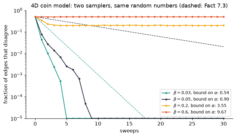
Look at the two regimes. For (teal, ink), disagreements vanish entirely within a few sweeps, below the dashed guarantee. (The plot floors exact zero at .) For and , Fact 7.2 gives no guarantee, and the disagreements never die. They fail in two different ways:
- At , below the jump, the two samplers disagree on about 40% of their face products too. Each sampler still forgets its start (chapter 4 checked this by other means). But this particular coupling no longer forces them together. A failed certificate is not proof of slow forgetting.
- At , past the jump, the samplers end up agreeing on about 99% of face products while disagreeing on half the labels. They have reached nearly the same class (chapter 1) by different labelings. A coupling that compares labels cannot see that two reframed labelings are "the same".
Recap. A coupling runs two random processes on shared randomness. With the best coupling at every update, the chance that two heat-bath samplers disagree at any edge shrinks by a factor per sweep. When the sampler forgets its start geometrically fast.
Check yourself
- In the proof, why is it important that the samplers use the best coupling rather than independent random numbers?
Answer
With independent draws, two identical conditional distributions would still give different labels most of the time, so disagreements would never die. The best coupling makes the disagreement probability equal to the distance between the conditional distributions, which is what the influences bound.
- On the coin model at , roughly how many sweeps does Fact 7.3 need before all labels agree with probability at least ?
Answer
. We need , so sweeps. In the plot it took fewer: the bound is a guarantee, not a prediction.
7.3 From forgetting to decorrelation
Forgetting in time (sweeps of a sampler) now gives forgetting in space (distance on the board). The trick: a correlation between and measures how much conditioning on moves the average of . Conditioning on is the same as reweighting the model by . A reweighted model is a new model whose conditional distributions agree with the old one at every edge that does not read. So we can couple a sampler of the old model with a sampler of the reweighted one. Their disagreements are created only on 's edges, and they fade with influence distance.
For a function of a labeling, write . Say reads a set of edges if it depends only on their labels.
Fact 7.4 (decorrelation). Suppose . Let read , let read , and let be the influence distance between and . Then the correlation of and is at most in absolute value.
In one line:
Proof.
Step 1 (reweight). Replace by ; this does not change the correlation. If the correlation is . Otherwise let be the model reweighted by , that is, . Then , and .
Step 2 (same conditionals off ). At an edge , the factor does not depend on . It cancels from the conditional distribution, so and have the same heat bath at .
Step 3 (couple). Run a heat-bath sampler of and one of , started from samples of and , so that at every time and . Use best couplings. An update at produces a disagreement with probability at most if , and at most if . Let
The sum converges because every row of sums to at most . Exactly as in Fact 7.3, the excess shrinks by a factor per sweep. So .
Step 4 (read off ). . Now let .
Step 5 (count paths). is a sum over chains of face-sharing steps from to , so it vanishes unless . Each power satisfies . So for .
Notice what the proof never used: reframings, the group structure, or the dimension. Only the sparsity of who-listens-to-whom (a bounded-degree influence graph) and the weakness of each link matter. (Probabilists call this Dobrushin's uniqueness theorem. Computer scientists know its relatives as "spatial mixing" and "correlation decay", the engine of several deterministic approximate-counting algorithms.)
Checking Fact 7.4 exactly. We need a model where correlations at long distances can be computed exactly, not sampled. The transfer matrix of chapter 5 does that. Take the 3D coin model, layered so that each layer is a torus. Its 18 layer edges give layer labelings, and the invariant functions form a subspace of dimension 1024. The helper below applies without ever writing it down, using two facts:
- with the step edges summed out, a slab reweights each layer edge independently;
- the invariant functions are spanned by products of labels along even subgraphs of the layer (every vertex touched an even number of times), because for an abelian group invariants are functions of loop products (glossary 3.5).
Its derivation is in the helper's comments.
# --- helpers: the exact transfer matrix of the 3D coin model on a W x W torus layer ----------------
# Layer labeling a in {+1,-1}^n (n = 2 W^2 layer edges). Summing the step edges over all their values is
# the same as summing over reframings of the upper layer (Fact 5.1), so on invariant functions
#     T = 2^(W^2) * D^(1/2) K D^(1/2),   K(a,b) = prod_e exp(-beta (1 - a_e b_e)),
# with D(a) = exp(-beta * total cost of the faces inside the layer) (split half and half between slabs).
# K is a tensor power of a 2x2 matrix, diagonal in the "parity" basis chi_S(a) = prod_{e in S} a_e,
# with eigenvalue (1+q)^(n-|S|) (1-q)^|S|, q = exp(-2 beta). chi_S is invariant exactly when S has even
# degree at every vertex. We apply K with a fast Walsh-Hadamard transform (n passes of sums/differences).

def layer_geometry(W):
    edges = [((x, y), mu) for x in range(W) for y in range(W) for mu in (0, 1)]
    eid = {e: i for i, e in enumerate(edges)}
    head = lambda v, mu: ((v[0] + (mu == 0)) % W, (v[1] + (mu == 1)) % W)
    faces = [[eid[((x, y), 0)], eid[(head((x, y), 0), 1)], eid[(head((x, y), 1), 0)], eid[((x, y), 1)]]
             for x in range(W) for y in range(W)]
    at_vertex = {}
    for (v, mu), i in eid.items():
        at_vertex.setdefault(v, []).append(i); at_vertex.setdefault(head(v, mu), []).append(i)
    return len(edges), faces, at_vertex

def walsh(f, n):
    x = f.reshape((2,) * n)
    for ax in range(n):
        a, b = np.take(x, 0, axis=ax), np.take(x, 1, axis=ax)
        x = np.stack([a + b, a - b], axis=ax)
    return x.reshape(-1)

class CoinLayerTransfer:
    """T / 2^(W^2) restricted to invariant functions of a W x W torus layer of the 3D coin model."""
    def __init__(self, W, beta):
        n, faces, at_vertex = layer_geometry(W)
        idx = np.arange(2 ** n, dtype=np.int64)
        bit = lambda i: np.int64(1) << (n - 1 - i)
        self.label = lambda i: 1 - 2 * ((idx & bit(i)) != 0)        # value of layer edge i, per labeling
        S_in = sum(1 - np.prod([self.label(e) for e in f], axis=0) for f in faces)
        self.Dh, self.n, self.faces = np.exp(-beta * S_in / 2), n, faces
        pop = lambda m: np.bitwise_count((idx & m).astype(np.uint64)).astype(np.int64)
        even = np.ones(2 ** n, dtype=bool)
        for es in at_vertex.values():
            even &= pop(np.bitwise_or.reduce([bit(e) for e in es])) % 2 == 0
        q, size = np.exp(-2 * beta), pop(np.int64(-1) & (2 ** n - 1))
        self.diag = even * (1 + q) ** (n - size) * (1 - q) ** size / 2 ** n
    def apply(self, f):
        return self.Dh * walsh(self.diag * walsh(self.Dh * f, self.n), self.n)
    def top(self, k=2):
        op = LinearOperator((2 ** self.n,) * 2, matvec=self.apply, dtype=float)
        vals, vecs = eigsh(op, k=k, which="LA")
        order = np.argsort(vals)[::-1]
        return vals[order], vecs[:, order]
First, a sanity check of the helper. The face product of one face inside layer 0, , is an invariant. On a board with infinitely many layers, the average of is , where is the top eigenvector and multiplies by (chapter 5, section 5.5). Fact 7.4 bounds the correlation by , with in 3D.
beta = 0.05
TL = CoinLayerTransfer(3, beta)
(lam0, _), vecs = TL.top()
psi0 = vecs[:, 0]
A = np.prod([TL.label(e) for e in TL.faces[0]], axis=0).astype(float)       # one face product
v, mean_A = A * psi0, psi0 @ (A * psi0)
alpha = 12 * np.tanh(beta)
print(f"beta = {beta}, alpha <= {alpha:.3f}")
for t in range(1, 3):
    v = TL.apply(v) / lam0
    corr = psi0 @ (A * v) - mean_A ** 2
    print(f"t = {t}: exact correlation {corr:.3e}   Fact 7.4 bound {16 * alpha ** t / (1 - alpha):.3e}")
print(f"tanh(beta)^4 = {np.tanh(beta) ** 4:.3e}")
beta = 0.05, alpha <= 0.600
t = 1: exact correlation 6.198e-06 Fact 7.4 bound 2.395e+01
t = 2: exact correlation 3.852e-11 Fact 7.4 bound 1.436e+01
tanh(beta)^4 = 6.229e-06
The exact correlation falls by a factor of about per layer. (Beyond it drops below rounding error.) The guaranteed rate is per layer, and the guaranteed constant is far above 1 at these distances. The bound is extremely generous, but it is a proof, and it holds for every board width at once. The factor has a simple meaning: to correlate a face in layer with one in layer , the model has to pass the information through the four side faces of the cube between them.
Recap. Reweighting by creates a model that agrees with the original everywhere except on 's edges. Coupling samplers of the two models shows that the disagreement leaks from to only along chains of influences, each costing a factor . So correlations decay like .
Check yourself
- Fact 7.4 has but not in the bound. Why the asymmetry?
Answer
Disagreements are created on , with probability at most 1 per edge. But we bound their arrival at each edge of by a sum over all sources, which is already included in . Then we add over the edges of that reads. (Applying the fact with and swapped gives the other version; use whichever is smaller.)
- Does Fact 7.4 say anything about non-invariant functions, such as a single label?
Answer
Yes. It holds for all functions, but for a single label it is vacuous: single labels average to zero (chapter 3), and so do their products at different edges. The real content is about invariants such as face products and loop observables.
7.4 From decorrelation to a gap
Chapter 5 showed, by experiment, that the gap is the rate at which layers forget each other. Now we can run that observation backwards as a proof. Decorrelation at rate per layer forces every level to sit at least above the lowest.
Fact 7.5 (a provable gap). Take a layered torus grid in dimensions whose layers are -dimensional tori of side . Let be any compact group and any face cost of spread . If , then every level of the transfer matrix satisfies for . In particular the gap is at least , for every width .
Proof. We write it for finite . For compact , replace sums by integrals; the Perron–Frobenius theorem for matrices is then replaced by its version for positive integral kernels (Jentzsch's theorem).
Step 1 (the top eigenvector is positive). Every entry is a sum of positive weights, and is symmetric (chapter 5). By the Perron–Frobenius theorem, is simple and has an eigenvector with every entry positive.
Step 2 (a test function for each level). Let be a unit eigenvector for , , so . Define the function of a layer labeling ; this is legal because . On a board with layers, the average of is . As , tends to . So the average tends to
and .
Step 3 (apply Fact 7.4). reads the layer edges of layer 0, and those of layer . A face touches at most two consecutive layers, so the influence distance between layer 0 and layer is at least . Fact 7.4 gives, uniformly in ,
Step 4 (take roots). Let : for every . Take -th roots and let : .
Step 4 is where the width disappears. grows with , but it is a constant in , and the -th root kills it. The rate only knows about one edge and its neighbors.
Now the comparison with exact gaps. For the 2D coin model chapter 5 gave . For the 3D coin model with layers, the helper computes it.
betas = np.geomspace(0.004, 1.0, 26)
E1_3d = []
for b in betas:
    (l0, l1), _ = CoinLayerTransfer(3, b).top()
    E1_3d.append(-np.log(l1 / l0))
E1_3d = np.array(E1_3d)
floor = lambda d: np.where(6 * (d - 1) * np.tanh(betas) < 1, -np.log(6 * (d - 1) * np.tanh(betas)), np.nan)
print("beta     exact E1 (3D, W=3)   proven floor (3D)")
for i in [0, 8, 12, 14]:
    print(f"{betas[i]:.4f}   {E1_3d[i]:8.3f}             {floor(3)[i]:.3f}")
beta exact E1 (3D, W=3) proven floor (3D)
0.0040 16.564 3.037
0.0234 11.264 1.270
0.0566 8.616 0.387
0.0881 7.294 nan
fig, ax = plt.subplots(figsize=(8, 4.4))
ax.plot(betas, -3 * np.log(np.tanh(betas)), color=viz.MUTED, lw=1.5, label="exact gap, 2D, $W=3$")
ax.plot(betas, E1_3d, "o-", ms=3, color=viz.INK, label="exact gap, 3D, $3\\times3$ layers")
ax.plot(betas, floor(2), color=viz.TEAL, lw=2.5, label="proven floor $\\ln(1/\\alpha)$, 2D (any $W$)")
ax.plot(betas, floor(3), color=viz.CORAL, lw=2.5, label="proven floor $\\ln(1/\\alpha)$, 3D (any $W$)")
ax.axvspan(betas[0], np.arctanh(1 / 12), color=viz.CORAL, alpha=0.08)
ax.set(xscale="log", ylim=(0, 18), xlabel=r"stiffness $\beta$", ylabel="gap $E_1$",
       title="Coin model: true gaps and the floor that Fact 7.5 proves")
ax.legend(fontsize=9); plt.show()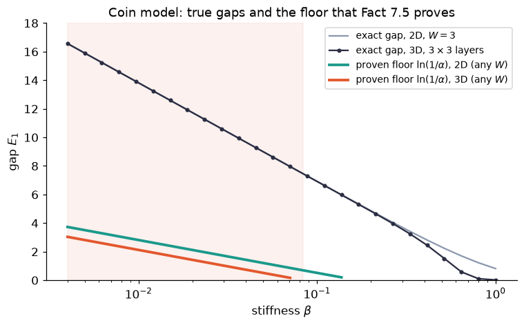
Look at the shaded region, where the 3D guarantee applies: the coral floor stays under the exact gap, as it must. It is far under, by a factor of about 8. The floor is crude but universal. It holds for every width at once and for every compact group with the same spread, and it knew nothing about this particular board beyond "each edge has 12 neighbors". As grows past , the floor drops to zero and the theorem says nothing. The true 3D gap keeps going, and becomes small near , where the 3D coin model has a jump of its own.
One more observation: at small the exact 3D gap is about , the same as the 2D gap with . The lightest state is a loop of length 3 wrapping around the layer. That is the "flux loop" of chapter 5, whose level grows with its length.
Recap. Each level is the decay rate of the correlation of a specific layer function, . Fact 7.4 bounds every such correlation by a constant times . Taking -th roots removes the constant, so for every and every width. The exact gaps of the coin model confirm the floor.
Check yourself
- Why do we need to be positive everywhere?
Answer
To divide by it: must be a genuine function of the layer labeling, with . Perron–Frobenius guarantees positivity because every entry of is positive.
- For 4D with , what does Fact 7.5 prove at ?
Answer
, so , and on every 4D torus grid, whatever its width. The correlation length is at most about 1 grid step.
- The 2D gap grows with . Is that consistent with a floor that does not depend on ?
Answer
Yes. A floor is only a lower bound, and for all . The floor cannot grow with because it is proved one edge at a time, without ever looking at the size of the layer.
7.5 Why this does not prove the Millennium gap
Fact 7.5 is a real theorem about lattice Yang–Mills. With on a 4D grid it is the small- entry "positive gap at small , proved" in chapter 6's status table, re-derived with a computer-science tool. Here is how far it reaches:
| Model (4D) | Spread | Fact 7.5 applies for our | physicists' | Where continuum physics is simulated () |
|---|---|---|---|---|
| coin | 2 | 0.056 | – | – |
| 4 | 0.028 | 0.056 | 2.3 – 3 | |
| 4.5 | 0.025 | 0.074 | 5.7 – 7 |
The gap between the last two columns is a factor of 40 to 100. But the true obstruction is not the size of the constants. There are three separate reasons, in increasing order of depth.
1. Influence grows with stiffness. At large each edge listens strongly to its neighbors, so . This is not only a weakness of the bound: as correlations reach further, the heat-bath sampler of chapter 4 really does slow down, because forgetting in space and forgetting in time go together. Sharper tools from computer science ("spectral independence", block dynamics, "high-dimensional expanders") push the threshold further. But they all certify the same kind of thing: correlations die within a bounded number of grid steps, with constants fixed in advance. Reason 3 shows why that kind of certificate must fail along the continuum path.
2. The board's geometry is not the issue. The hint "use expander graphs" points at a real principle, local-to-global: a local condition on a sparse graph ( on the influence graph) gives a global conclusion. But Fact 7.5 already works on the 4D grid, which is a poor expander: a box of side has vertices but only about boundary edges. Expansion of the board plays no role. What matters is the weakness of each link, and that is exactly what fails at large .
3. The scale problem (the deep one). The Millennium gap is not "the gap is positive". From chapter 6: as the grid spacing , with growing like for , one needs
A bound like , a constant in grid units, would give if it held along the continuum path: every particle infinitely heavy, and the limit would be trivial. So a proof must show that the gap in grid units shrinks, exponentially in , at the rate set by asymptotic freedom, and no faster. That is a statement connecting all scales at once. No single-scale argument can deliver it.
What a proof would need, in our terms. Group the grid into blocks of side . The distribution of suitable block labels is again a model, with a more complicated but still local cost. Asymptotic freedom says its effective stiffness decreases as the blocks grow. So the natural plan, Balaban's, is:
- (UV) Control the blocking from spacing
up to a fixed physical block size
,
uniformly as
.
This is what the 2026 proof does, up to a reference
scale where the stiffness equals a fixed
(see
notes/yang_mills_existence_2026.md). - (Crossover) Keep blocking until the effective stiffness falls below the threshold of a Fact-7.5-type theorem, while keeping the effective cost local.
- (IR) Apply a Fact-7.5-type theorem, generalized to local costs on several faces (the proof goes through verbatim: influence is still a sum over shared terms of ), to the blocked model. Then show that fine-scale observables, given the block labels, are themselves local. The result would be a gap of at least in physical units.
The first step is done. The last is this chapter, plus a locality lemma. The middle step is the open problem. The UV methods work by expanding around consistent labelings, which needs large stiffness. The IR method needs stiffness below about 0.03. Between them is the smooth crossover you saw in chapter 6's Creutz plot, where the model is neither nearly consistent nor nearly independent, and no known method controls it. The 2026 proof itself avoids this region. Per the committee's assessment, its large-volume step rests on compactness, flip-positivity and the transfer-matrix representation, and it proves no clustering of correlations. That is why it obtains existence along a subsequence, a mixture of phases, and no gap.
Recap. Fact 7.5 covers only below a few hundredths, far from where the continuum lives. Beyond that, influence is too strong. More fundamentally, the Millennium gap needs the grid-unit gap to shrink at exactly the asymptotic-freedom rate, which is a multi-scale statement. The missing piece is control of the crossover between the near-consistent regime (handled by the 2026 existence proof) and the near-independent regime (handled by this chapter).
Check yourself
- Suppose someone proves for all in 4D . Would that solve the Millennium gap?
Answer
No, it would refute the expected continuum limit. Along the continuum path the gap in physical units would be , so the limiting theory would have no particles at all. Physicists expect like .
- What lower bound on in grid units, for large , would a solution need to prove (for , leading order)?
Answer
for some and all large , along with the existence of the limit. Then stays bounded below. (An upper bound of the same form, needed for a non-trivial limit, is expected from asymptotic freedom.)
Chapter recap
- The influence is the most the heat-bath distribution at can move when the label at changes. The influence number is the largest total influence on one edge. On a grid, (Facts 7.1, 7.2).
- A coupling runs two random processes on shared randomness. With best couplings, two heat-bath samplers disagree at any edge with probability at most after sweeps (Fact 7.3). This is the path-coupling argument for rapid mixing.
- Reweighting by changes the model only on 's edges. Coupling the two models gives correlations at most (Fact 7.4).
- Testing with turns decorrelation into a floor under every level: for every width, every compact group, every dimension (Fact 7.5). Checked against exact 2D and 3D coin-model gaps.
- For 4D the theorem applies for . The continuum needs with a gap that shrinks at the asymptotic-freedom rate, a multi-scale statement no single-scale argument can give.
- The missing step is the crossover between the regime the 2026 existence proof controls and the regime this chapter controls.
Dictionary
| Our term | Other names |
|---|---|
| distance between distributions | total variation distance |
| best coupling | maximal (optimal) coupling |
| influence | Dobrushin interdependence matrix |
| Dobrushin's uniqueness condition; in physics, a "high-temperature" or "strong-coupling" condition | |
| two samplers on the same random numbers | synchronous coupling; path coupling (Bubley–Dyer) |
| sampler forgets geometrically | rapid mixing of Glauber dynamics |
| correlations decay with influence distance | spatial mixing, correlation decay, uniqueness of the Gibbs measure |
| Fact 7.5 for | mass gap at strong coupling (Osterwalder–Seiler 1978, by cluster expansion) |
| blocking the grid | renormalization group (block-spin transformation); Balaban's program |
| the crossover | the intermediate-coupling regime; the gap between perturbative and strong-coupling control |
What's next
This chapter ends the elementary road. Two directions continue it. On
the computer-science side: can spectral independence or block
(multi-scale) dynamics give a gap that shrinks at a controlled
rate for the 3D coin model, where the answer is known from its exact
relation to the 3D Ising model? On the physics side: the 2026 proof's
blocking machinery, read in our terms, is the natural place to look for
the crossover step. Read the notes in
notes/yang_mills_existence_2026.md with this chapter's
three-step plan in mind. The research memo
notes/crossover/README.md takes the middle step further: it
shows that the simplest blocking scheme runs on the curvature of
(and stalls for the circle), measures how wide the crossover really is,
and lists what a certificate tight enough to cross it would need.